Diffusion models in SO3 space

One typical way to represent the structure of proteins is to use the position of alpha carbon and the rotation matrix of each residue. So the diffusion process on the space of alpha carbon is simple Euclidean space, but the diffusion process on the rotation matrix ($SO(3)$ space) is non-Euclidean.

In this notebook, I will show the general formulation of diffusion models in $SO3$ space.

Score function and noise adding process

Just like the diffusion process in euclidean space, the core part of the diffusion process includes the score function and noise adding process. So to understand the diffusion process in $SO3$ space, I will first show the noise adding process (or random walk) in the 3D space.

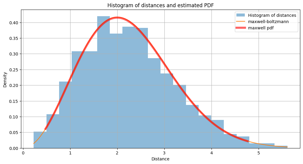
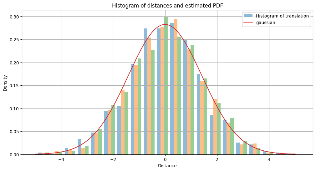
Random walk in 3D space

We generate stepsize from a gaussian distribution with std= 0.1 in x,y,z direction, after 200 steps, we found that the distance from origin follows from the Maxwell-Boltzmann distribution with std = $\sqrt{0.1\ast 200}$

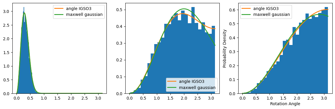
Random walk in SO3 space

Likewise in the 3D cases, we can do the random walk in $SO3$ space by sampling angles from gaussian distributions and compose them with Lie algebra bases. To write it formally, $$\begin{array}{c}{r}^{(t+1)}=\exp \left\{\sum _{d=1}^3{ϵ}_d{G}_d\right\}{r}^t\end{array}$$

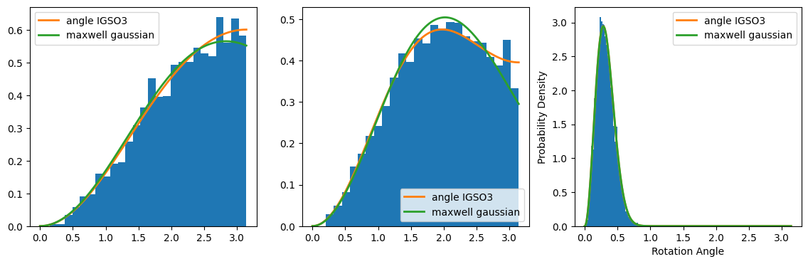
We found out that the angle distribution of this noise adding process follows the distribution called IGSO3 distribution, which writes: $$\begin{array}{c}f(\omega ,\sigma )=\frac{1-\cos \omega }{\pi }\sum _{l=0}^{\infty }(2l+1)e^{-l(l+1){\sigma }^2/2}\frac{\sin \left(\left(l+\frac{1}{2}\right)\omega \right)}{\sin (\omega /2)}\end{array}$$

Denoising dynamics in general and in SO3 space

The denoising dynamics in general can be formulated into a reverse SDE corresponding to a forward SDE in continuous form. A remarkable result from Anderson states that, the reverse SDE equation for a forward SDE process: $$\begin{array}{c}\mathrm{d}\mathbf{x}=\mathbf{f}(\mathbf{x},t)\mathrm{d}t+g(t)\mathrm{d}\mathbf{w}\end{array}$$ can be modeled as: $$\begin{array}{c}\mathrm{d}\mathbf{x}=\left[\mathbf{f}(\mathbf{x},t)-g(t{)}^2{\nabla }_{\mathbf{x}}\log p_t(\mathbf{x})\right]\mathrm{d}t+g(t)\mathrm{d}\overline{\mathbf{w}}\end{array}$$ Note that this formulation is in Euclidean space, in $SO(3)$ case, we have to use the formulation in Lie algebra space, then exponentiate back to $SO(3)$ space.

To write it more explicitly, we can write the random walk in Lie algebra space as: $$\begin{array}{c}{L}_{t+1}=L_t+{\beta }_{\mathbf{t}}\cdot \mathbf{G}\end{array}$$ where ${\beta }_{\mathbf{t}}$ is sampled from three gaussian distribution with standard deviation $\sqrt{{\sigma }_t^2-{\sigma }_{t-1}^2}$, $\mathbf{G}$ is the Three Lie algebra matrix.

Then the reverse process of this SDE in Lie algebra space is: $$\begin{array}{c}{L}_t=L_{t+1}+({\sigma }_t^2-{\sigma }_{t-1}^2){\nabla }_{L^{(t)}}\log q\left(L_t\right)+\sqrt{{\sigma }_t^2-{\sigma }_{t-1}^2}{ϵ}_{\mathbf{t}}\cdot \mathbf{G}\end{array}$$ Exponentiate back to the $SO(3)$ matrix, we have the reverse process in $SO(3)$ space: $$\begin{array}{c}{r}^{(t-1)}=\exp \left\{\left({\sigma }_t^2-{\sigma }_{t-1}^2\right){\nabla }_{r^{(t)}}\log q\left(r^{(t)}\right)+\sqrt{{\sigma }_t^2-{\sigma }_{t-1}^2}\sum _{d=1}^3{ϵ}_d{G}_d\right\}{r}^t,\end{array}$$ where $q(r^{(t)}$ is the probability density of matrix $r^{(t)}$ of the marginal distribution in the forward process. Now it is only a matter of calculating the expression ${\nabla }_{r^{(t)}}\log q\left(r^{(t)}\right)$, which is also called the score function.

Score function in SO3 space

The score function in SO3 space can be written using the chain rule: $$\begin{array}{c}{\nabla }_r\log q\left(r^{(t)}\right)={{\nabla }_r\omega \left({\bar{r}}^{\top }{r}^{(t)}\right)\frac{d}{d\omega }[\log \frac{f\left(\omega ;{\sigma }_t^2\right)}{1-\cos \omega }]|}_{\omega =\omega \left({\bar{r}}^{\top }r\right)}\end{array}$$

Write the gradient of the rotation angle in compact form: Write in a compact form, using the identity $$\begin{array}{c}\hat{r}v=\log (\hat{r}{e}^v{\hat{r}}^{\top })\end{array}$$ $$\begin{array}{c}{\nabla }_r\omega \left({\hat{r}}^{\top }r\right)=\frac{\hat{r}\log ({\hat{r}}^{\top }r)}{\omega ({\hat{r}}^{\top }r)}=\frac{\log (r{\hat{r}}^{\top })}{\omega ({\hat{r}}^{\top }r)}=\frac{r\log ({\hat{r}}^{\top }r)}{\omega ({\hat{r}}^{\top }r)}\end{array}$$

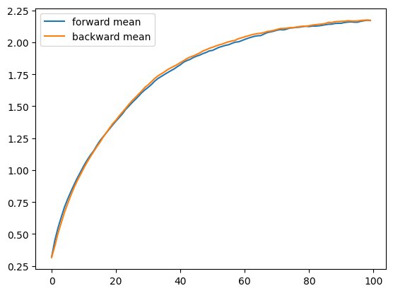
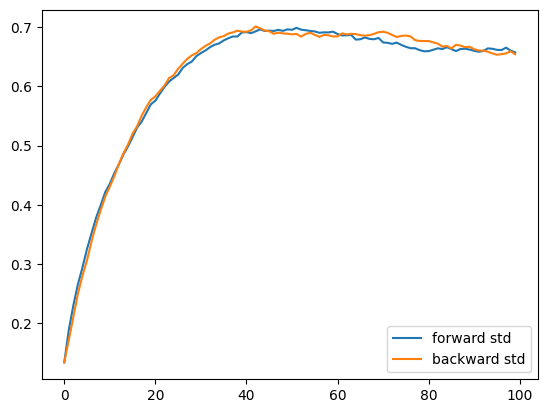
Mean and std of the forward and backward process

We can plot the mean and std of the forward and backward process, and find them to be consistent.

We can also plot the rotation angle distribution along the denoising process.