Geometry-Aware Fourier Neural Operator (Geo-FNO)

代码

文本

©️Copyright @ Authors

日期：2023-05-09
共享协议：本作品采用知识共享署名-非商业性使用-相同方式共享 4.0 国际许可协议进行许可。

Abstract

深度学习代理模型在求解偏微分方程(PDEs)方面显示出了良好的前景。其中,傅里叶神经算子(FNO)在各种PDEs(如流体流动)上实现了良好的精度,并且与数值求解器相比速度显著加快。然而,FNO使用快速傅里叶变换(FFT),仅限于具有均匀网格的矩形域。在这项工作中,作者提出了一个新的框架,即Geo-FNO,用于求解任意几何形状上的PDEs。Geo-FNO学习将输入(物理)域(可能是不规则的)变形为具有均匀网格的潜在空间。在latent space中应用了带有FFT的FNO模型。由此产生的Geo-FNO模型既具有FFT的计算效率,又具有处理任意几何形状的灵活性。这样的Geo-FNO在输入格式方面也很灵活,即点云、网格和设计参数都是有效的输入。考虑了多种PDEs, 如弹性方程、塑性方程、欧拉方程和纳维-斯托克斯方程,以及正向建模和逆向设计问题。与标准数值求解器相比,Geo-FNO的速度提高了10⁵倍,与现有的基于机器学习的PDE求解器(如标准FNO)相比,精度提高了两倍。

本文为边看边学系列，即笔者一边看paper一边学😂。notebook的前半部分为笔记，后半部分为示例代码。 完整运行代码只需要几分钟。

Paper: https://arxiv.org/abs/2207.

代码

文本

Paper Notes

Questions & Motivations

由于求解PDE在整个问题域上经常遇到的网格非均匀性，不管是自适应网格细化或者是动网格都无法解决传统数据方法在复杂几何上计算速度很慢的问题。
神经算子（Neural Operator）旨在以网格不变的方式直接学习偏微分方程的解算子，它对于离散化具有不变性，因此更适合求解偏微分方程^†。然而FNO是通过FFT实现的，因此它只能用于具有均匀网格的矩形域。当将其应用于不规则域形状时，以前的工作通常将域嵌入到更大的矩形域中。然而，这种嵌入效率较低且浪费，特别是对于高度不规则的几何形状。先前在均匀与非均匀网格之间的插值方法，也可能会导致比较大的插值误差。

Propositions
- 一种感知的FNO框架（Geo-FNO），适用于任意几何形状。
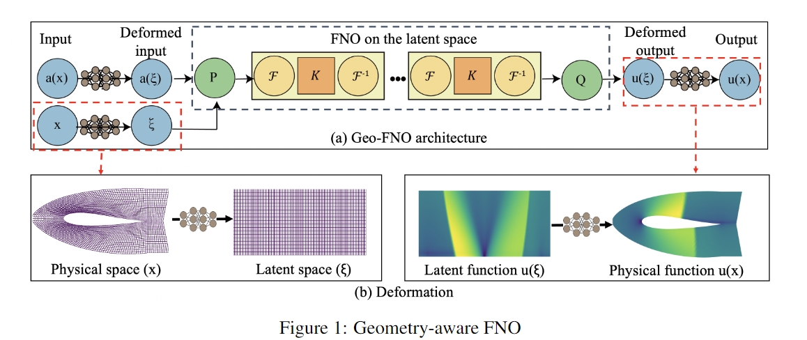
- Geo-FNO 将不规则输入域变形为可以应用 FFT 的均匀潜在网格。这种变形可以通过 FNO 架构以端到端的方式学习。用一个神经网络对变形进行建模。
- 在正向建模和逆向设计任务中对弹性、塑性、欧拉和纳维-斯托克斯方程的不同几何形状进行实验。与数值求解器相比，Geo-FNO 的加速比高达10⁵，并且与之前基于插值的方法相比，误差降低了一半。

原则上，这个Geo-FNO框架可以直接拓展到一般拓扑。即对复杂的输入拓扑分解为规则的子域。此外，也可以拓展到包括PDE约束的PINO（physics-informed neural operator）。

†：关于FNO的更多内容可以参考Notebook。FNO具有优越的成本精度权衡，它通过快速傅里叶变换 (FFT) 实现一系列计算全局卷积算子的层，然后混合频域权重和傅里叶逆变换。这些全局卷积算子中散布着诸如 GeLU 之类的非线性变换。通过组合全局卷积算子和非线性激活，FNO 可以逼近高度非线性和非局部解算子。 FNO 及其变体能够模拟许多偏微分方程，例如纳维-斯托克斯方程和地震波，进行高分辨率天气预报，并以前所未有的成本精度权衡来预测二氧化碳迁移。

下图为Geo-FNO的模型框架：

代码

文本

Preliminaries

为了简化和约束问题，一些假设：

假设所有域都是嵌入在某些背景欧几里得空间 Ω（例如 R3）中的有界可定向流形。
假设初始条件和边界条件都是固定的。
只考虑稳态解。

计算域或者几何的形状可以通过网格、函数和设计参数等多种方式给出。最常见的形式就是网格（点云）。函数的例子比如2D表面的边界函数，或者是SDF。设计参数可以是高、宽、体积、角度和半径等，这种形式适合一些设计问题。

代码

文本

Model: Geometry-Aware Fourier Neural Operator

核心思想：将物理空间变形为规则的计算空间，以便在其上进行FFT。

形式上，需要找到输入域 D_a和单位环面 D_c=[0,1]^d之间的微分同胚变形 φ_a（映射）。计算空间网格 D_c在所有输入域 D_a之间共享，它满足均匀网格和标准傅里叶基。一旦确定了映射 φ_a，就可以在物理空间上产生自适应网格和变形傅里叶基。这样的映射可作用于函数、方程组和系统。
关于将物理空间上的函数变换到计算域谱空间上的推导，读者可以阅读原文章3.2节的内容。
值得注意的是，如果输入是规则的结构化网格，那么Geo-FNO简化为标准FNO。而对于哪些输入域具有不规则拓扑，与环面不同胚的PDEs问题，需要首先将输入域嵌入到更大的规则域中。这种嵌入对应于传统谱求解器中使用的傅里叶连续技术（Fourier continuation）。

代码

文本

Results

文中将Geo-FNO与其他机器学习模型在多种不同几何形状的PDEs进行了比较。这里我们以流体力学的NS方程为例，结果如下：

翼型流场和管流场结果绘图：

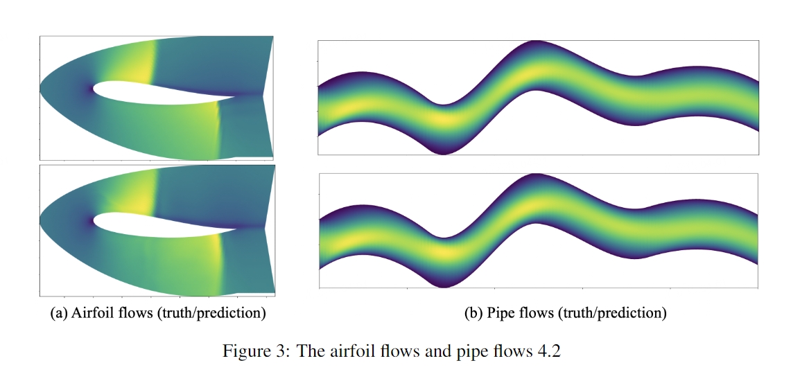
Geo-FNO可以应用于不规则域和非均匀网格。它比现有基于 ML 的 PDE 求解器（例如标准 FNO 和 UNet）以及无网格方法（例如图神经算子 (GNO) 和 DeepONet）上的直接插值更准确。同时，Geo-FNO 保持了标准 FNO 的速度，在所有实验中每个实例的推理时间约为 0.01 秒，它可以将机翼问题的数值求解器加速高达 10⁵ 倍。 下表为在机翼问题上各种模型的比较：

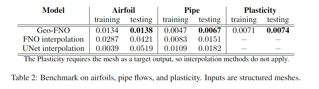
值得注意的是，作者在文章中提到：与具有固定启发式变形（R 网格）和（O 网格）的 Geo-FNO 相比，具有学习变形的 Geo-FNO 具有更好的精度。当然，这种结论针对的是非结构化网格。

Inverse design

关于反问题，这里主要指逆向设计。当 Geo-FNO 模型训练完成后，可以通过直接优化设计参数来达到设计目标。下图就是一个反问题的例子：

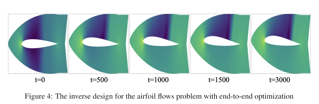
这里设定的设计目标是最小化阻力和最大化升力。首先训练从输入网格到输出压力场的模型映射，并以端到端的方式优化样条节点。从图中可以看出，经过优化迭代，得到的翼型变得不对称，上弯度更大，这增加了升力系数，符合物理直觉。数值求解器的模拟与预测相符，阻力为 0.04，升力为 0.29。

所有实验均在单个Nvidia 3090 GPU上执行。如无特别提及，均用 500 个epoch训练所有模型，初始学习率为 0.001，每 100 个epoch衰减一半。使用相对 L2 误差进行训练和测试。

代码

文本

Codes

下面我们以Elasticity (弹性问题)为例，展示Geo-FNO模型的框架和训练过程。

在 Bohrium Notebook 界面，你可以点击界面上方蓝色按钮 开始连接，选择 bohrium-notebook:2023-03-26 镜像及 c12_m92_1 * NVIDIA V100 节点配置，稍等片刻即可运行。

Code from Github

代码

文本

[1]

import torch.nn.functional as F

import matplotlib.pyplot as plt

from timeit import default_timer

import sys

sys.path.append('/bohr/geofno-wukj/v2/elasticity/')

from utilities3 import *

from Adam import Adam

已隐藏输出

代码

文本

[2]

def set_seed(seed):

torch.manual_seed(seed)

np.random.seed(seed)

torch.cuda.manual_seed(seed)

torch.backends.cudnn.deterministic = True

set_seed(0)

已隐藏输出

代码

文本

Fourier layer

代码

文本

[3]

class SpectralConv2d(nn.Module):

def __init__(self, in_channels, out_channels, modes1, modes2, s1=32, s2=32):

super(SpectralConv2d, self).__init__()

"""

2D Fourier layer. It does FFT, linear transform, and Inverse FFT.

"""

self.in_channels = in_channels

self.out_channels = out_channels

self.modes1 = modes1 # Number of Fourier modes to multiply, at most floor(N/2) + 1

self.modes2 = modes2

self.s1 = s1

self.s2 = s2

self.scale = (1 / (in_channels * out_channels))

self.weights1 = nn.Parameter(

self.scale * torch.rand(in_channels, out_channels, self.modes1, self.modes2, dtype=torch.cfloat))

self.weights2 = nn.Parameter(

self.scale * torch.rand(in_channels, out_channels, self.modes1, self.modes2, dtype=torch.cfloat))

# Complex multiplication

def compl_mul2d(self, input, weights):

# (batch, in_channel, x,y ), (in_channel, out_channel, x,y) -> (batch, out_channel, x,y)

return torch.einsum("bixy,ioxy->boxy", input, weights)

def forward(self, u, x_in=None, x_out=None, iphi=None, code=None):

batchsize = u.shape[0]

# Compute Fourier coeffcients up to factor of e^(- something constant)

if x_in == None:

u_ft = torch.fft.rfft2(u)

s1 = u.size(-2)

s2 = u.size(-1)

else:

u_ft = self.fft2d(u, x_in, iphi, code)

s1 = self.s1

s2 = self.s2

# Multiply relevant Fourier modes

# print(u.shape, u_ft.shape)

factor1 = self.compl_mul2d(u_ft[:, :, :self.modes1, :self.modes2], self.weights1)

factor2 = self.compl_mul2d(u_ft[:, :, -self.modes1:, :self.modes2], self.weights2)

# Return to physical space

if x_out == None:

out_ft = torch.zeros(batchsize, self.out_channels, s1, s2 // 2 + 1, dtype=torch.cfloat, device=u.device)

out_ft[:, :, :self.modes1, :self.modes2] = factor1

out_ft[:, :, -self.modes1:, :self.modes2] = factor2

u = torch.fft.irfft2(out_ft, s=(s1, s2))

else:

out_ft = torch.cat([factor1, factor2], dim=-2)

u = self.ifft2d(out_ft, x_out, iphi, code)

return u

def fft2d(self, u, x_in, iphi=None, code=None):

# u (batch, channels, n)

# x_in (batch, n, 2) locations in [0,1]*[0,1]

# iphi: function: x_in -> x_c

batchsize = x_in.shape[0]

N = x_in.shape[1]

device = x_in.device

m1 = 2 * self.modes1

m2 = 2 * self.modes2 - 1

# wavenumber (m1, m2)

k_x1 = torch.cat((torch.arange(start=0, end=self.modes1, step=1), \

torch.arange(start=-(self.modes1), end=0, step=1)), 0).reshape(m1,1).repeat(1,m2).to(device)

k_x2 = torch.cat((torch.arange(start=0, end=self.modes2, step=1), \

torch.arange(start=-(self.modes2-1), end=0, step=1)), 0).reshape(1,m2).repeat(m1,1).to(device)

# print(x_in.shape)

if iphi == None:

x = x_in

else:

x = iphi(x_in, code)

# print(x.shape)

# K = <y, k_x>, (batch, N, m1, m2)

K1 = torch.outer(x[...,0].view(-1), k_x1.view(-1)).reshape(batchsize, N, m1, m2)

K2 = torch.outer(x[...,1].view(-1), k_x2.view(-1)).reshape(batchsize, N, m1, m2)

K = K1 + K2

# basis (batch, N, m1, m2)

basis = torch.exp(-1j * 2 * np.pi * K).to(device)

# Y (batch, channels, N)

u = u + 0j

Y = torch.einsum("bcn,bnxy->bcxy", u, basis)

return Y

def ifft2d(self, u_ft, x_out, iphi=None, code=None):

# u_ft (batch, channels, kmax, kmax)

# x_out (batch, N, 2) locations in [0,1]*[0,1]

# iphi: function: x_out -> x_c

batchsize = x_out.shape[0]

N = x_out.shape[1]

device = x_out.device

m1 = 2 * self.modes1

m2 = 2 * self.modes2 - 1

# wavenumber (m1, m2)

k_x1 = torch.cat((torch.arange(start=0, end=self.modes1, step=1), \

torch.arange(start=-(self.modes1), end=0, step=1)), 0).reshape(m1,1).repeat(1,m2).to(device)

k_x2 = torch.cat((torch.arange(start=0, end=self.modes2, step=1), \

torch.arange(start=-(self.modes2-1), end=0, step=1)), 0).reshape(1,m2).repeat(m1,1).to(device)

if iphi == None:

x = x_out

else:

x = iphi(x_out, code)

# K = <y, k_x>, (batch, N, m1, m2)

K1 = torch.outer(x[:,:,0].view(-1), k_x1.view(-1)).reshape(batchsize, N, m1, m2)

K2 = torch.outer(x[:,:,1].view(-1), k_x2.view(-1)).reshape(batchsize, N, m1, m2)

K = K1 + K2

# basis (batch, N, m1, m2)

basis = torch.exp(1j * 2 * np.pi * K).to(device)

# coeff (batch, channels, m1, m2)

u_ft2 = u_ft[..., 1:].flip(-1, -2).conj()

u_ft = torch.cat([u_ft, u_ft2], dim=-1)

# Y (batch, channels, N)

Y = torch.einsum("bcxy,bnxy->bcn", u_ft, basis)

Y = Y.real

return Y

已隐藏输出

代码

文本

FNO

代码

文本

[4]

class FNO2d(nn.Module):

def __init__(self, modes1, modes2, width, in_channels, out_channels, is_mesh=True, s1=40, s2=40):

super(FNO2d, self).__init__()

"""

The overall network. It contains 4 layers of the Fourier layer.

1. Lift the input to the desire channel dimension by self.fc0 .

2. 4 layers of the integral operators u' = (W + K)(u).

W defined by self.w; K defined by self.conv .

3. Project from the channel space to the output space by self.fc1 and self.fc2 .

input: the solution of the coefficient function and locations (a(x, y), x, y)

input shape: (batchsize, x=s, y=s, c=3)

output: the solution

output shape: (batchsize, x=s, y=s, c=1)

"""

self.modes1 = modes1

self.modes2 = modes2

self.width = width

self.is_mesh = is_mesh

self.s1 = s1

self.s2 = s2

self.fc0 = nn.Linear(in_channels, self.width) # input channel is 3: (a(x, y), x, y)

self.conv0 = SpectralConv2d(self.width, self.width, self.modes1, self.modes2, s1, s2)

self.conv1 = SpectralConv2d(self.width, self.width, self.modes1, self.modes2)

self.conv2 = SpectralConv2d(self.width, self.width, self.modes1, self.modes2)

self.conv3 = SpectralConv2d(self.width, self.width, self.modes1, self.modes2)

self.conv4 = SpectralConv2d(self.width, self.width, self.modes1, self.modes2, s1, s2)

self.w1 = nn.Conv2d(self.width, self.width, 1)

self.w2 = nn.Conv2d(self.width, self.width, 1)

self.w3 = nn.Conv2d(self.width, self.width, 1)

self.b0 = nn.Conv2d(2, self.width, 1)

self.b1 = nn.Conv2d(2, self.width, 1)

self.b2 = nn.Conv2d(2, self.width, 1)

self.b3 = nn.Conv2d(2, self.width, 1)

self.b4 = nn.Conv1d(2, self.width, 1)

self.fc1 = nn.Linear(self.width, 128)

self.fc2 = nn.Linear(128, out_channels)

def forward(self, u, code=None, x_in=None, x_out=None, iphi=None):

# u (batch, Nx, d) the input value

# code (batch, Nx, d) the input features

# x_in (batch, Nx, 2) the input mesh (sampling mesh)

# xi (batch, xi1, xi2, 2) the computational mesh (uniform)

# x_in (batch, Nx, 2) the input mesh (query mesh)

if self.is_mesh and x_in == None:

x_in = u

if self.is_mesh and x_out == None:

x_out = u

grid = self.get_grid([u.shape[0], self.s1, self.s2], u.device).permute(0, 3, 1, 2)

u = self.fc0(u)

u = u.permute(0, 2, 1)

uc1 = self.conv0(u, x_in=x_in, iphi=iphi, code=code)

uc3 = self.b0(grid)

uc = uc1 + uc3

uc = F.gelu(uc)

uc1 = self.conv1(uc)

uc2 = self.w1(uc)

uc3 = self.b1(grid)

uc = uc1 + uc2 + uc3

uc = F.gelu(uc)

uc1 = self.conv2(uc)

uc2 = self.w2(uc)

uc3 = self.b2(grid)

uc = uc1 + uc2 + uc3

uc = F.gelu(uc)

uc1 = self.conv3(uc)

uc2 = self.w3(uc)

uc3 = self.b3(grid)

uc = uc1 + uc2 + uc3

uc = F.gelu(uc)

u = self.conv4(uc, x_out=x_out, iphi=iphi, code=code)

u3 = self.b4(x_out.permute(0, 2, 1))

u = u + u3

u = u.permute(0, 2, 1)

u = self.fc1(u)

u = F.gelu(u)

u = self.fc2(u)

return u

def get_grid(self, shape, device):

batchsize, size_x, size_y = shape[0], shape[1], shape[2]

gridx = torch.tensor(np.linspace(0, 1, size_x), dtype=torch.float)

gridx = gridx.reshape(1, size_x, 1, 1).repeat([batchsize, 1, size_y, 1])

gridy = torch.tensor(np.linspace(0, 1, size_y), dtype=torch.float)

gridy = gridy.reshape(1, 1, size_y, 1).repeat([batchsize, size_x, 1, 1])

return torch.cat((gridx, gridy), dim=-1).to(device)

已隐藏输出

代码

文本

Geometric Fourier Transform

代码

文本

[5]

class IPHI(nn.Module):

def __init__(self, width=32):

super(IPHI, self).__init__()

"""

inverse phi: x -> xi

"""

self.width = width

self.fc0 = nn.Linear(4, self.width)

self.fc_code = nn.Linear(42, self.width)

self.fc_no_code = nn.Linear(3*self.width, 4*self.width)

self.fc1 = nn.Linear(4*self.width, 4*self.width)

self.fc2 = nn.Linear(4*self.width, 4*self.width)

self.fc3 = nn.Linear(4*self.width, 2)

self.center = torch.tensor([0.5,0.5], device="cuda").reshape(1,1,2)

self.B = np.pi*torch.pow(2, torch.arange(0, self.width//4, dtype=torch.float, device="cuda")).reshape(1,1,1,self.width//4)

def forward(self, x, code=None):

# x (batch, N_grid, 2)

# code (batch, N_features)

# some feature engineering

angle = torch.atan2(x[:,:,1] - self.center[:,:, 1], x[:,:,0] - self.center[:,:, 0])

radius = torch.norm(x - self.center, dim=-1, p=2)

xd = torch.stack([x[:,:,0], x[:,:,1], angle, radius], dim=-1)

# sin features from NeRF

b, n, d = xd.shape[0], xd.shape[1], xd.shape[2]

x_sin = torch.sin(self.B * xd.view(b,n,d,1)).view(b,n,d*self.width//4)

x_cos = torch.cos(self.B * xd.view(b,n,d,1)).view(b,n,d*self.width//4)

xd = self.fc0(xd)

xd = torch.cat([xd, x_sin, x_cos], dim=-1).reshape(b,n,3*self.width)

if code!= None:

cd = self.fc_code(code)

cd = cd.unsqueeze(1).repeat(1,xd.shape[1],1)

xd = torch.cat([cd,xd],dim=-1)

else:

xd = self.fc_no_code(xd)

xd = self.fc1(xd)

xd = F.gelu(xd)

xd = self.fc2(xd)

xd = F.gelu(xd)

xd = self.fc3(xd)

return x + x * xd

已隐藏输出

代码

文本

Configs

代码

文本

[6]

Ntotal = 2000

ntrain = 1000

ntest = 200

batch_size = 20

learning_rate_fno = 0.001

learning_rate_iphi = 0.0001

epochs = 201

modes = 12

width = 32

已隐藏输出

代码

文本

load data and data normalization

代码

文本

[7]

PATH_Sigma = '/bohr/geofno-wukj/v2/elasticity_data/Meshes/Random_UnitCell_sigma_10.npy'

PATH_XY = '/bohr/geofno-wukj/v2/elasticity_data/Meshes/Random_UnitCell_XY_10.npy'

PATH_rr = '/bohr/geofno-wukj/v2/elasticity_data/Meshes/Random_UnitCell_rr_10.npy'

input_rr = np.load(PATH_rr)

input_rr = torch.tensor(input_rr, dtype=torch.float).permute(1,0)

input_s = np.load(PATH_Sigma)

input_s = torch.tensor(input_s, dtype=torch.float).permute(1,0).unsqueeze(-1)

input_xy = np.load(PATH_XY)

input_xy = torch.tensor(input_xy, dtype=torch.float).permute(2,0,1)

train_rr = input_rr[:ntrain]

test_rr = input_rr[-ntest:]

train_s = input_s[:ntrain]

test_s = input_s[-ntest:]

train_xy = input_xy[:ntrain]

test_xy = input_xy[-ntest:]

print(train_rr.shape, train_s.shape, train_xy.shape)

train_loader = torch.utils.data.DataLoader(torch.utils.data.TensorDataset(train_rr, train_s, train_xy), batch_size=batch_size, shuffle=True)

test_loader = torch.utils.data.DataLoader(torch.utils.data.TensorDataset(test_rr, test_s, test_xy), batch_size=batch_size, shuffle=False)

torch.Size([1000, 42]) torch.Size([1000, 972, 1]) torch.Size([1000, 972, 2])

代码

文本

Training and evaluation

代码

文本

[9]

model = FNO2d(modes, modes, width, in_channels=2, out_channels=1).cuda()

model_iphi = IPHI().cuda()

print(count_params(model), count_params(model_iphi))

optimizer_fno = Adam(model.parameters(), lr=learning_rate_fno, weight_decay=1e-4)

scheduler_fno = torch.optim.lr_scheduler.CosineAnnealingLR(optimizer_fno, T_max = 200)

optimizer_iphi = Adam(model_iphi.parameters(), lr=learning_rate_iphi, weight_decay=1e-4)

scheduler_iphi = torch.optim.lr_scheduler.CosineAnnealingLR(optimizer_iphi, T_max = 200)

myloss = LpLoss(size_average=False)

N_sample = 1000

for ep in range(epochs):

model.train()

t1 = default_timer()

train_l2 = 0

train_reg = 0

for rr, sigma, mesh in train_loader:

rr, sigma, mesh = rr.cuda(), sigma.cuda(), mesh.cuda()

optimizer_fno.zero_grad()

optimizer_iphi.zero_grad()

out = model(mesh, code=rr, iphi=model_iphi)

loss = myloss(out.view(batch_size, -1), sigma.view(batch_size, -1))

loss.backward()

optimizer_fno.step()

optimizer_iphi.step()

train_l2 += loss.item()

scheduler_fno.step()

scheduler_iphi.step()

model.eval()

test_l2 = 0.0

with torch.no_grad():

for rr, sigma, mesh in test_loader:

rr, sigma, mesh = rr.cuda(), sigma.cuda(), mesh.cuda()

out = model(mesh, code=rr, iphi=model_iphi)

test_l2 += myloss(out.view(batch_size, -1), sigma.view(batch_size, -1)).item()

train_l2 /= ntrain

test_l2 /= ntest

t2 = default_timer()

if ep%50==0:

print(f'Epoch:{ep} Time:{t2 - t1:.3f} Train loss:{train_l2:.3f}, Test loss:{test_l2:.3f}')

if ep%100==0:

# torch.save(model, '../model/elas_v2_'+str(ep))

# torch.save(model_iphi, '../model/elas_v2_iphi_'+str(ep))

XY = mesh[-1].squeeze().detach().cpu().numpy()

truth = sigma[-1].squeeze().detach().cpu().numpy()

pred = out[-1].squeeze().detach().cpu().numpy()

lims = dict(cmap='RdBu_r', vmin=truth.min(), vmax=truth.max())

fig, ax = plt.subplots(nrows=1, ncols=3, figsize=(12, 4))

ax[0].scatter(XY[:, 0], XY[:, 1], 100, truth, edgecolor='w', lw=0.1, **lims)

ax[1].scatter(XY[:, 0], XY[:, 1], 100, pred, edgecolor='w', lw=0.1, **lims)

ax[2].scatter(XY[:, 0], XY[:, 1], 100, truth - pred, edgecolor='w', lw=0.1, **lims)

fig.show()

# plt.savefig('output.png')

1482657 47234
Epoch:0 Time:1.135 Train loss:0.463, Test loss:0.290
Epoch:50 Time:1.128 Train loss:0.027, Test loss:0.033
Epoch:100 Time:1.135 Train loss:0.018, Test loss:0.028
Epoch:150 Time:1.136 Train loss:0.013, Test loss:0.025
Epoch:200 Time:1.139 Train loss:0.012, Test loss:0.025

代码

文本

[ ]

代码

文本

Geometry-Aware Fourier Neural Operator (Geo-FNO)

Abstract

Paper Notes

Questions & Motivations

Propositions

Preliminaries

Model: Geometry-Aware Fourier Neural Operator

Results

Inverse design

Codes

Fourier layer

FNO

Geometric Fourier Transform

Configs

load data and data normalization

Training and evaluation