
新建
seq2seq improvement
 微信用户7sxQ
更新于 2024-12-26
推荐镜像 :Basic Image:bohrium-notebook:2023-03-26
推荐机型 :c2_m4_cpu
赞
调库
代码
文本
[ ]
import torch
import torch.nn as nn
import torch.optim as optim
from torch.nn.utils.rnn import pad_sequence
import torch.nn.functional as F
import random
import numpy as np
import pandas as pd
import matplotlib.pyplot as plt
from sklearn.preprocessing import MinMaxScaler
from pyswarm import pso
代码
文本
使用GPU提高运行效率
代码
文本
[ ]
device = 'cuda' if torch.cuda.is_available() else 'cpu' # 如果电脑有GPU,则在GPU上运算,否则在CPU上运算
代码
文本
定义数据分割函数
代码
文本
[ ]
def split_list_by_value(lst):
result = []
temp = []
for i in range(len(lst)):
if lst[i] != 0:
temp.append(lst[i])
if i == len(lst)-1 or lst[i] != lst[i+1]:
result.append(temp)
temp = []
return result
def split_list_by_lengths(lst, lengths):
result = []
start = 0
for length in lengths:
result.append(lst[start:start+length])
start += length
return result
代码
文本
电压电流数据处理(优化点1:多学习一个特征脉冲电流数据,有助于提高预测准确性和理解电池系统的行为)
代码
文本
[ ]
total_num = 222
train_size = 194
test_size = 28
CC_input = []
cyc_len = []
baty_lst = [2,3,4,6,7,8]
for i in baty_lst:
CC_data = pd.read_csv(f"/pycharm project/pythonProject/dataset/Capacity data/Data_Capacity_25C0{i}.csv")
cycle_num = CC_data.iloc[:, 1:2]["cycle number"].tolist()
vol_all = CC_data.iloc[:, 3:4]['Ewe/V'].tolist()
cur_all=CC_data.iloc[:,4:5][' I/mA'].tolist()#这里多学习一个特征,即脉冲电流数据,让模型预测的更准
cyc = split_list_by_value(cycle_num)
if i == 7:
cyc = cyc[:-7]
cyc_len.append(len(cyc))
lengths = [len(sublist) for sublist in cyc]
vol_list = split_list_by_lengths(vol_all, lengths)
cur_list= split_list_by_lengths(cur_all, lengths)
tensor_vol = [torch.tensor(sublist).view(-1, 1) for sublist in vol_list] # [N, 1]
tensor_cur = [torch.tensor(sublist).view(-1, 1) for sublist in cur_list] # [N, 1]
padded_vol = pad_sequence(tensor_vol, batch_first=True, padding_value=0) # [batch_size, max_len, 1]
padded_cur = pad_sequence(tensor_cur, batch_first=True, padding_value=0) # [batch_size, max_len, 1]
#print(padded_vol.shape)
combined_features = torch.cat((padded_vol, padded_cur), dim=-1)#将每个时间步的电压和电流数据被组合在一起,形成一个新的张量
print("Combined features shape:", combined_features.shape)#验证数据是否按照预期的方式被合并
for feature in combined_features:
CC_input.append(feature[:1654])
print(len(CC_input), cyc_len)
代码
文本
以25C0{2}号电池举例,画出它的部分脉冲电压及电流数据
代码
文本
[ ]
pulse=pd.read_csv(f"/pycharm project/pythonProject/dataset/Capacity data/Data_Capacity_25C0{2}.csv")
plt.figure(figsize=(12, 4.5))
plt.subplot(1, 2, 1)
plt.plot(pulse[0:8050][' I/mA'], 'r')
plt.title('Pulse Current')
plt.xlabel('Time(s)')
plt.ylabel('Current(mA)')
plt.subplot(1, 2, 2)
plt.plot(pulse[0:8050]['Ewe/V'], 'b')
plt.title('Pulse Voltage')
plt.xlabel('Time(s)')
plt.ylabel('Voltage(V)')
plt.show()
代码
文本
分割encoder输入数据为训练集和测试集
代码
文本
[ ]
indices = list(range(len(CC_input)))
random.shuffle(indices)
CC_input_scaled = []
for data in CC_input:
data = np.array(data) # 转换为数组并去除多余的维度
# 将数据重新形状为(-1, 1)使其适应MinMaxScaler的输入格式
scaled_data = scaler.fit_transform(data.reshape(-1, 2))
# 将标准化后的数据转换为Tensor并添加到列表中
CC_input_scaled.append(torch.tensor(scaled_data).view(1,-1, 2))
train_indices = indices[:train_size]
test_indices = indices[train_size:]
encoder_input_train=[CC_input_scaled[i] for i in train_indices]
encoder_input_test=[CC_input_scaled[i] for i in test_indices]
代码
文本
EIS数据处理
代码
文本
[ ]
decoder_input = []
decoder_target = []
cyc_tot = 0
EIS_list = [[[0 for i in range(240)] for j in range(2)] for r in range(222)]
lst = [1, 4, 5, 9]
for k in baty_lst:
EIS_tot = []
for i in lst:
EIS = pd.read_csv(f"/pycharm project/pythonProject/dataset/EIS data/EIS_state_{i}_25C0{k}.csv")
cyc_n = cyc_len[baty_lst.index(k)]
#print(cyc_n)
EIS_tot.append(EIS.iloc[:, 3:7][" Re(Z)/Ohm"].tolist()[0:60 * cyc_n])
EIS_tot.append(EIS.iloc[:, 4:7][" -Im(Z)/Ohm"].tolist()[0:60 * cyc_n])
cyc_tot += cyc_n
EIS_totm = [[e2 for e2 in e1] for e1 in EIS_tot]
print(np.array(EIS_totm).shape, cyc_tot)
lengths = [60 for i in range(cyc_n)]
# print(lengths)
for i in range(4):
EIS_R = split_list_by_lengths(EIS_totm[2 * i], lengths)
EIS_I = split_list_by_lengths(EIS_totm[2 * i + 1], lengths)
for j in range(cyc_tot - cyc_n, cyc_tot, 1):
EIS_list[j][0][60 * i:60 * (i + 1)] = EIS_R[j - cyc_tot + cyc_n]
EIS_list[j][1][60 * i:60 * (i + 1)] = EIS_I[j - cyc_tot + cyc_n]
EIS_list = [np.array(t).squeeze().T for t in EIS_list]
print(np.array(EIS_list)[0].shape)
代码
文本
EIS数据标准化
代码
文本
[ ]
scaler = MinMaxScaler(feature_range=(0, 1))
EIS_scaled = []
for i in range(len(EIS_list)):
EIS_data = EIS_list[i] # 获取EIS数据
# 使用MinMaxScaler对每个EIS数据进行标准化
scaled_EIS = scaler.fit_transform(EIS_data) # 将数据标准化到[0, 1]
EIS_scaled.append(torch.tensor(scaled_EIS).float()) # 转换为Tensor并添加到列表中
print("Standardized EIS data:", np.array(EIS_scaled).shape)
代码
文本
处理Decoder的输入数据和输出的目标数据
代码
文本
[ ]
decoder_target = [torch.tensor(t).float().view(1,240, 2) for t in EIS_scaled]
decoder_input = [torch.ones(1,240,2) for t in EIS_scaled]
decoder_input_train = [decoder_input[i] for i in train_indices]
decoder_target_train = [decoder_target[i] for i in train_indices]
decoder_input_test = [decoder_input[i] for i in test_indices]
decoder_target_test = [decoder_target[i] for i in test_indices]
print(decoder_input[0].shape)
代码
文本
粒子群优化算法(注意:实际运行时,不用运行这一段代码)
代码
文本
[ ]
# def optimize_function(params):
# hidden_size = int(params[0]) # 隐藏层单元数
# learning_rate = params[1] # 学习率
# encoder = Encoder(hidden_size=hidden_size).to(device)
# decoder = Decoder(hidden_size=hidden_size).to(device)
# model = EncoderDecoder(encoder, decoder).to(device)
# optimizer = optim.Adam(model.parameters(), lr=learning_rate)
# criterion = nn.MSELoss().to(device)
# num_epochs = 1500
# batch_size = 4
# train_losses = [] # 记录每个epoch的训练损失
# for epoch in range(num_epochs):
# epoch_loss = 0.0
# teacher_forcing_ratio = max(0.5 * (1 - epoch / num_epochs), 0.0)
# use_teacher_forcing = True
# for batch_idx in range(0, train_size, batch_size):
# batch_encoder_input = torch.cat(encoder_input_train[batch_idx:batch_idx + batch_size], dim=0).to (device)
# batch_decoder_input = torch.cat(decoder_input_train[batch_idx:batch_idx + batch_size], dim=0).to (device)
# batch_decoder_target = torch.cat(decoder_target_train[batch_idx:batch_idx + batch_size], dim=0).to (device)
# optimizer.zero_grad()
# outputs = model(batch_encoder_input, batch_decoder_input, use_teacher_forcing).to (device)
# loss = criterion(outputs, batch_decoder_target)
# if torch.isnan(loss).any() or loss is None or loss == float('inf'):
# print(f"Invalid loss at epoch {epoch}, batch {batch_idx}")
# return float('inf') # Avoid passing None or invalid loss to PSO
# loss.backward()
# optimizer.step()
# epoch_loss += loss.item()
# train_losses.append(epoch_loss / (train_size / batch_size))
# if (epoch + 1) % 20 == 0:
# mean_mse = epoch_loss / (train_size / batch_size)
# rmse = mean_mse ** 0.5
# print(f"Epoch [{epoch + 1}/{num_epochs}], Loss: {mean_mse:.8f}, RMSE: {rmse}")
# return mean_mse if mean_mse is not None else float('inf')
# #scheduler.step(epoch_loss)
# lb = [128, 1e-5] # 下边界 [隐藏层单元数,学习率]
# ub = [512, 1e-2] # 上边界 [隐藏层单元数,学习率]
# # 使用PSO优化
# best_params, _ = pso(optimize_function, lb, ub, swarmsize=5, maxiter=10)
# # 输出最优的超参数
# best_hidden_size = int(best_params[0])
# best_lr = best_params[1]
# print(f"Optimized hidden size: {best_hidden_size}")
# print(f"Optimized learning rate: {best_lr}")
代码
文本
模型的定义,优化点2:超参数优化,LSTM隐藏单元数的调整(采用PSO算法得到的最佳隐藏单元数)
代码
文本
[ ]
# define encoder
class Encoder(nn.Module):
def __init__(self):
super(Encoder, self).__init__()
self.lstm = nn.LSTM(2, 282, batch_first=True, num_layers=2, dropout=0.5)#输入维度由只有电压变为电压+电流,另外将LSTM隐藏单元数调整至最优(PSO粒子群优化算法寻得的)
def forward(self, x):
_, (h_n, c_n) = self.lstm(x)
return h_n, c_n
# define decoder
class Decoder(nn.Module):
def __init__(self):
super(Decoder, self).__init__()
self.lstm = nn.LSTM(2, 282, batch_first=True, num_layers=2) # 增加单元数
self.dense = nn.Linear(282, 2) # 输出维度为2
def forward(self, x, hidden):
x, _ = self.lstm(x, hidden)
x = self.dense(x)
return x
# define Encoder-Decoder model
class EncoderDecoder(nn.Module):
def __init__(self, encoder, decoder):
super(EncoderDecoder, self).__init__()
self.encoder = encoder
self.decoder = decoder
def forward(self, encoder_input, decoder_input, use_teacher_forcing):
hidden = self.encoder(encoder_input)
if use_teacher_forcing:
output = self.decoder(decoder_input, hidden)
else:
batch_size, seq_len, _ = decoder_input.size()
output = torch.zeros_like(decoder_input)
decoder_input_t = decoder_input[:, 0, :]
for t in range(seq_len):
decoder_output_t = self.decoder(decoder_input_t.unsqueeze(1), hidden)
output[:, t, :] = decoder_output_t.squeeze(1)
decoder_input_t = decoder_output_t.squeeze(1)
return output
代码
文本
构造模型
代码
文本
[ ]
encoder = Encoder()
decoder = Decoder()
model = EncoderDecoder(encoder, decoder).to (device)
print(model)
代码
文本
训练过程及记录,优化点3:超参数优化,学习率优化(采用PSO算法得到的最佳学习率)
代码
文本
[ ]
criterion = nn.MSELoss().to (device)
optimizer = optim.Adam(model.parameters(), lr=0.000388)#同样是通过粒子群优化算法PSO寻得的最优learning rate
num_epochs = 500
batch_size = 10
train_losses = [] # 记录每个epoch的训练损失
for epoch in range(num_epochs):
epoch_loss = 0.0
teacher_forcing_ratio = max(0.5 * (1 - epoch / num_epochs), 0.0)
use_teacher_forcing = True
for batch_idx in range(0, train_size, batch_size):
batch_encoder_input = torch.cat(encoder_input_train[batch_idx:batch_idx + batch_size], dim=0).to (device)
batch_decoder_input = torch.cat(decoder_input_train[batch_idx:batch_idx + batch_size], dim=0).to (device)
batch_decoder_target = torch.cat(decoder_target_train[batch_idx:batch_idx + batch_size], dim=0).to (device)
optimizer.zero_grad()
outputs = model(batch_encoder_input, batch_decoder_input, use_teacher_forcing).to (device)
loss = criterion(outputs, batch_decoder_target)
loss.backward()
optimizer.step()
epoch_loss += loss.item()
train_losses.append(epoch_loss / (train_size / batch_size))
if (epoch + 1) % 20 == 0:
mean_mse = epoch_loss / (train_size / batch_size)
rmse = mean_mse ** 0.5
print(f"Epoch [{epoch + 1}/{num_epochs}], Loss: {mean_mse:.8f}, RMSE: {rmse}")
代码
文本
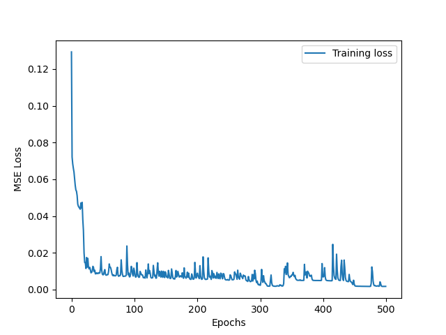
将训练过程中loss变化画出来
代码
文本
[ ]
plt.plot(train_losses, label='Training loss')
plt.xlabel('Epochs')
plt.ylabel('MSE Loss')
plt.legend()
plt.show()
代码
文本
代码
文本
利用训练好的模型进行测试
代码
文本
[ ]
model.eval().to (device)
test_losses = []
for batch_idx in range(0, test_size, batch_size):
batch_encoder_input = torch.cat(encoder_input_test[batch_idx:batch_idx+batch_size], dim=0).to (device)
batch_decoder_input = torch.cat(decoder_input_test[batch_idx:batch_idx+batch_size], dim=0).to (device)
batch_decoder_target = torch.cat(decoder_target_test[batch_idx:batch_idx+batch_size], dim=0).to (device)
with torch.no_grad():
outputs = model(batch_encoder_input, batch_decoder_input, use_teacher_forcing).to (device)
loss = criterion(outputs, batch_decoder_target).to (device)
test_losses.append(loss.item())
mean_mse = np.mean(test_losses)
test_rmse = mean_mse ** 0.5
print(f"Test Loss: {mean_mse:.4f} Test RMSE: {test_rmse:.4f}")
代码
文本
将测试集的预测结果与target value进行比较
代码
文本
[ ]
predict_outputs = outputs[0].view(1, 240, 2).tolist()
predict_data = np.array(predict_outputs).squeeze().T
decoder_target = batch_decoder_target[0].view(1, 240, 2).tolist()
target_data = np.array(decoder_target).squeeze().T
for i in range(4):
if i == 1:
label_p = 'Predict EIS'
label_t = 'Target EIS'
else:
label_p = None
label_t = None
plt.plot(predict_data[0][60 * i:60 * (i + 1)], predict_data[1][60 * i:60 * (i + 1)], 'ro-', label=label_p)
plt.plot(target_data[0][60 * i:60 * (i + 1)], target_data[1][60 * i:60 * (i + 1)], 'bo-', label=label_t)
plt.xlabel('Z_re')
plt.ylabel('Z_im')
plt.legend()
plt.show()
代码
文本

代码
文本
将四个状态分开画
代码
文本
[ ]
plt.figure(figsize=(11, 25))
title_name = [1, 4, 5, 9]
for i in range(4):
label_p = 'Predict EIS'
label_t = 'Target EIS'
plt.subplot(5, 2, i + 1)
plt.plot(predict_data[0][60 * i:60 * (i + 1)], predict_data[1][60 * i:60 * (i + 1)], 'ro-', label=label_p)
plt.plot(target_data[0][60 * i:60 * (i + 1)], target_data[1][60 * i:60 * (i + 1)], 'bo-', label=label_t)
titname = title_name[i]
plt.title(f"state {titname}")
plt.xlabel('Z_re')
plt.ylabel('Z_im')
plt.legend()
plt.show()
代码
文本

代码
文本
计算R2并绘图
代码
文本
[ ]
def r2_score(y_true, y_pred):
ss_total = np.sum((y_true - np.mean(y_true))**2)
ss_res = np.sum((y_true - y_pred)**2)
r2 = 1 - (ss_res / ss_total)
return r2
r2_r = 0
r2_i = 0
for i in range(4):
r2_r += r2_score(target_data[0][60*i:60*(i+1)], predict_data[0][60*i:60*(i+1)])/4
r2_i += r2_score(target_data[1][60*i:60*(i+1)], predict_data[1][60*i:60*(i+1)])/4
print(f"R2 real score:{r2_r.item():.4f}",f"R2 imaginary score:{r2_i.item():.4f}")
for i in range(4):
if i == 0:
plt.plot(target_data[0][60*i:60*(i+1)],target_data[0][60*i:60*(i+1)],'c-', linewidth=2, label='ground truth')
label_p = f'R2_real score:{r2_r:.4f}'
else:
label_p = None
plt.plot(target_data[0][60*i:60*(i+1)],predict_data[0][60*i:60*(i+1)],'mo', markerfacecolor='none', label=label_p)
plt.xlabel('real_true')
plt.ylabel('real_pred')
plt.title('Z real R2')
plt.legend()
plt.show()
for i in range(4):
if i == 0:
plt.plot(target_data[1][60*i:60*(i+1)],target_data[1][60*i:60*(i+1)],'c-', linewidth=2, label='ground truth')
label_p = f'R2_image score:{r2_i:.4f}'
else:
label_p = None
plt.plot(target_data[1][60*i:60*(i+1)],predict_data[1][60*i:60*(i+1)],'mo', markerfacecolor='none', label=label_p)
plt.xlabel('real_true')
plt.ylabel('real_pred')
plt.title('Z image R2')
plt.legend()
plt.show()
代码
文本


代码
文本
点个赞吧