Bohrium
robot
新建

空间站广场

论文
Notebooks
比赛
课程
Apps
我的主页
我的Notebooks
我的论文库
我的足迹

我的工作空间

任务
节点
文件
数据集
镜像
项目
数据库
公开
DMFF算法改进:在固定半径近邻搜索算法上的尝试 - DP_NBLIST
分子动力学
力场
分子动力学力场
yifeng_zhao
发布于 2024-05-06
推荐镜像 :Third-party software:dmff:1.0.0
推荐机型 :c16_m32_cpu
赞 1
6
3
一、固定半径近邻搜索
a. 定义
b. 应用场景
二、DP_NBLIST
a. Motivation
b. 结构设计
c. 三类算法实现
1. The Linked Cell Method
2. The Octree Method
3. The Hash-based Method
d. 应用案例
三、分析测试
a. 准确率测试
b. 效率测试
1. 线程调整
2. 性能趋势对比
3. Heatmap对比
c. 与DMFF的耦合
四、规律总结
a. CPU架构计算
b. GPU架构计算
c. 异构计算

一、固定半径近邻搜索

a. 定义

固定半径近邻搜索(Fixed-radius Neighbor Search)是一种邻居搜索算法,旨在查找数据集中距离指定目标在一固定半径范围内的所有对象。具体来说,它不仅要查找距离最近的邻居,还需要找到指定半径内的所有邻居对象(如r图1,左侧)。

查询到的邻居信息会以临近表(Neighbor List)的形式进行保存(如r图1,右侧)。通常,它会按照原子序号进行排布,并依次存储各粒子的邻居信息。

alt image.png
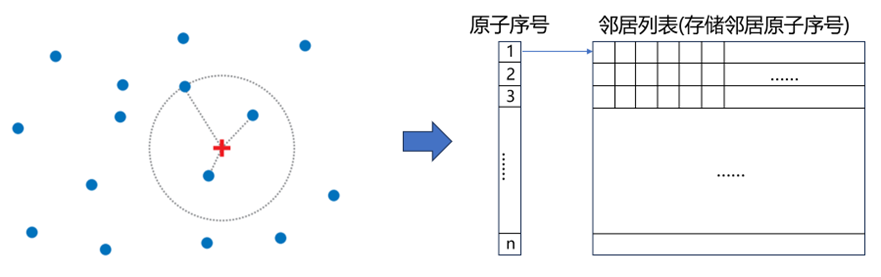
图1 固定半径邻居搜索及邻居表。其中左侧为一示例系统,红色十字为目标对象,圆形范围内的粒子即为其固定半径内近邻。

b. 应用场景

该算法在诸多领域中均有广泛使用,例如分子动力学模拟(MD),离散元方法(DEM),蒙特卡罗方法(MCS)和地理信息系统(GIS)等。 一个典型的应用是在MD之中,用于计算某特定粒子的邻居,并以此计算对应的相互作用力,形成相应的动力学行为。

在这些使用场景中,涉及的空间类型各异,但大致可以分为三类,即稠密空间、稀疏空间和非均一空间。稠密空间通常指是在特定区域内,对象之间的距离较小,对象数量相对较多,密集地堆积在一起形成连续的分布的空间;稀疏空间则指的是在特定区域内,对象之间的距离较大,对象数量相对较少的空间。此外,还存在一类具有不同大小对象的空间即非均一空间,通过一些技术,如stencil模板、动态调整等,可以将其归类为前两种空间类型之一。

alt

图2 主要空间类型

从应用角度而言,建立一个适用于多种场景、跨平台、高效的通用固定半径邻居搜索算法库,可以为不同领域的研究人员提供一种统一的工具,不仅能够降低开发和维护成本,还可以促进知识交流和跨领域合作,为科学和工程的创新提供便利。为此我们开发了DP-NBLIST。

代码
文本

二、DP_NBLIST

a. Motivation

该library旨在提供一种高性能、跨平台的固定半径近邻搜索算法实现。它包含三种适用于不同空间类型的搜索算法,支持CPU和GPU两种类型的运算。它对于输入输出格式进行了特别规约,以适配绝大多数仿真框架。

b. 结构设计

DP-NBLIST由三大模块构成(如图3):

(a)域模块:处理与仿真空间(域)的相关信息,包括空间的几何尺寸(size)和形状(angle),以及输入坐标的周期性规约(Warp函数)以及距离计算(calDistance)。

(b)邻近表模块:辅助邻近信息的构建和管理,包括它的构建(Build),更新(Update)和重置(Reset)。

(c)搜索算法模块:主要包含三种邻近搜索(Neighbor Search)的算法的CPU和GPU实现。

alt

图3 DP-NBLIST的三大主要模块

c. 三类算法实现

下面将对DP-NBLIST包含的三种算法进行简要说明,更多算法细节可参考我们的后续论文 。

在正式介绍算法细节之前,让我们设想一下最直觉的Neighbor Search算法:对于一个粒子系统,构建系统中每个粒子的固定半径邻居关系,需要遍历其所有潜在邻居粒子(即剩余的所有粒子),然后检验两者间的特征距离是否满足在指定半径之内(截断半径,cut-off radius - rc),以此为基准构建Neighbor List。

上述过程主要包含两步:(1)查找潜在邻居粒子,(2)判断潜在邻居粒子是否为真正邻居。显然上述算法具有的时间复杂度,并不适于大规模场景。对此,各类高效率Neighbor Search算法应运而生。这些算法在结构上具有相似性,即在步骤(1)中进行拓展优化,使用各种方法来提高查找潜在邻居粒子的效率。

1. The Linked Cell Method

Linked Cell方法是一种基于网格(Cell)的近邻搜索方法。它包含三个步骤(如图4):(1)使用Cell进行空间划分,(2)基于Cell进行潜在邻居粒子的查找,(3)判断潜在邻居粒子是否为真正邻居。

该方法可以将特定粒子的潜在邻居,有效的高效地缩减为其所在Cell的邻近Cell中的粒子(2D为9个邻接Cells,3D则为27个邻接Cells,如图4, b)。

alt

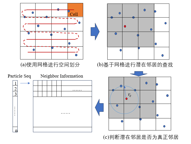
局限:在稀疏空间(存在对于大量空网格的随机读取)和rc较小(划分Cell过多,以[50,50,50]空间大小、rc = 1为例,需要划分125000个Cell)的场景下,性能表现不佳。

图4 Cell List近邻搜索算法

2. The Octree Method

Octree方法在步骤上与Linked Cell类似,区别主要在于空间划分。Octree方法使用了八叉树数据结构对系统中的粒子进行重组,以实现对于空间的划分。如图5 (a),此处以4个粒子一组构建八叉树,然后以层次地构建划分空间,然后相邻距离进行潜在邻居的查找。

alt

图5 基于Octree的近邻搜索算法

局限:在中等稠密空间和rc居中的场景下(此时建树较为昂贵,而树结构带来的潜在邻居查找效率优势不明显),性能表现不佳。

3. The Hash-based Method

Hash-based方法也是一种基于Cell的搜索算法。与Linked Cell不同,它使用Morton码对空间进行划分(如图5,a)。Morton码是一种空间填充曲线,能够将多维空间中的点交错相邻的映射到一维空间,常用于近似邻居搜索算法。这种划分方式能够使多维空间中相邻的数据在低维编码中也相对接近,使得数据在存储时处于相邻或连续的内存地址上,充分利用硬件缓存(Cache)和顺序读取的优势,显著提高总体效率。

alt

图5 基于Hash关系的近邻搜索算法

此外,我们对存储的数据结构也进行了优化。如图6 (a),我们在构建空间划分时,并不存储Cell中的所有粒子,而是在排序的基础上,仅存储每个Cell中起始和末尾粒子的序号,以进一步加强数据的关联性。在读取时(如图6 b),则使用顺序填充的方法,准确读取所有粒子。

alt

图6 基于Hash关系近邻搜索算法的数据结构

局限:在稀疏空间和rc较小的场景下(包含附加的数据排序和处理步骤),性能表现不佳。

代码
文本

d. 应用案例

此处将通过一个实例,来说明如何使用DP-NBLIST。

此处的模块编译于Github Link,模块使用pybind11进行封装,python环境版本3.10。

初步文档可见于Link

模块包含六种可选算法:"Linked_Cell-CPU", "Linked_Cell-GPU", "Octree-CPU", "Octree-GPU", "Hash-CPU"以及"Hash-GPU"。

注意GPU算法需要在包含GPU的环境中运行,且需要安装相关支持包(详见文档)。

代码
文本
[5]
import sys
import imp
import platform
import psutil
import numpy as np
# !pip install matplotlib
import matplotlib.pyplot as plt

# 读取CPU平台信息
cpu_info = platform.processor()
print("CPU information:", cpu_info)

current_freq = psutil.cpu_freq().current / 1000
max_freq = psutil.cpu_freq().max / 1000
min_freq = psutil.cpu_freq().min / 1000
print("Current CPU frequency:", current_freq, "GHz")

# 检验python版本
print("Python version:", sys.version)

# 导入 .so file
nblist_module = imp.load_dynamic('nblist', '/personal/nblist.cpython-310-x86_64-linux-gnu.so')
nblist_module.set_num_threads(10) # 设置线程数
print(nblist_module.get_max_threads()) # 查看最大线程数
print(dir(nblist_module)) # 查看有哪些方法

# 生成均匀随机数据
def generate_random_uniform_inputs(num_particles, domain_size):
inputs = []

for _ in range(num_particles):
input_temp = [
np.random.uniform(0., domain_size[0]),
np.random.uniform(0., domain_size[1]),
np.random.uniform(0., domain_size[2])
]
inputs.append(input_temp)
return np.array(inputs)

# 生成聚集随机数据
def generate_random_gaussian_inputs(num_particles, domain_size, num_centers = 2):
inputs = []
centers = []

for _ in range(num_centers):
centers.append([
np.random.uniform(5., domain_size[0]-5),
np.random.uniform(5., domain_size[1]-5),
np.random.uniform(5., domain_size[2]-5)
])
print(centers)
for _ in range(num_particles // num_centers):
for i in range(num_centers):
inputs.append([
np.random.normal(centers[i], 5.0),
np.random.normal(centers[i], 5.0)
])
return np.array(inputs)

def plot_dataset(dataset):
x = dataset[:, 0]
y = dataset[:, 1]
z = dataset[:, 2]

fig = plt.figure()
ax = fig.add_subplot(111, projection='3d')
ax.scatter(x, y, z, c='b', marker='o')
ax.set_xlabel('X Label')
ax.set_ylabel('Y Label')
ax.set_zlabel('Z Label')
plt.show()

# A showcase
domain_size = [50, 50, 50]
angle = [90, 90, 90]
num_particles_s = 1000
rc_s = 1

dataset_s = generate_random_uniform_inputs(num_particles_s, [50,50,50])
plot_dataset(dataset_s)

# 调用模块
box = nblist_module.Box(domain_size, angle)
nb_alg = nblist_module.NeighborList("Linked_Cell-CPU")
nb_alg.build(box, dataset_s, rc_s)
nb_list = nb_alg.get_neighbor_pair()
print(f"搜索结果:{nb_list}")
CPU information: x86_64
Current CPU frequency: 2.5000080000000007 GHz
Python version: 3.10.13 (main, Sep 11 2023, 13:21:10) [GCC 11.2.0]
10
['Box', 'NeighborList', '__doc__', '__file__', '__loader__', '__name__', '__package__', '__spec__', 'get_max_threads', 'set_num_threads']
搜索结果:[[  1 289]
 [  8 499]
 [ 16 402]
 [ 99 220]
 [155 848]
 [164 939]
 [220  99]
 [228 892]
 [243 912]
 [260 950]
 [289   1]
 [321 959]
 [370 884]
 [402  16]
 [403 455]
 [416 500]
 [455 403]
 [499   8]
 [500 416]
 [780 819]
 [819 780]
 [848 155]
 [884 370]
 [892 228]
 [912 243]
 [919 932]
 [932 919]
 [939 164]
 [950 260]
 [959 321]]
代码
文本

三、分析测试

a. 准确率测试

此处的准确率计算基于Asap3进行。

代码
文本
[21]
# Evalution of accuracy
# ! pip install asap3
import asap3
import ase
from ase import Atoms
import imp
import numpy as np
import imp

# 导入 .so 文件
nblist_module = imp.load_dynamic('nblist', '/personal/nblist.cpython-310-x86_64-linux-gnu.so')

# 生成均匀分布随机数据集
def generate_random_uniform_inputs(num_particles, domain_size):
inputs = []

for _ in range(num_particles):
input_temp = [
np.random.uniform(0., domain_size[0]),
np.random.uniform(0., domain_size[1]),
np.random.uniform(0., domain_size[2])
]
inputs.append(input_temp)
return np.array(inputs)

# 准确率分析
def evalute_accuracy(nb_alg1, nb_alg2, num_particles, rc):
sign = True
for i in range(num_particles):
set1 = nb_alg1.get_neighbors(i)
set2, _, _= nb_alg2.get_neighbors(i)
if set(set1) != set(set2):
print("error in %d, seq-%d" % (num_particles, i))
print(len(set(set1)))
print(len(set(set2)))
sign = False
if sign:
print(f"Pass the accuracy test of rc-{rc}!", )
else:
print(f"Fail the accurcy test of rc-{rc}!")
return sign


# domain信息
domain_size = [50, 50, 50]
angle = [90, 90, 90]
num_particles_a = 1000
rc_a = 2.1

dataset_a = generate_random_uniform_inputs(num_particles_a, [50,50,50])

# asap3
atoms = Atoms(f'{int(num_particles_a)}N', positions=dataset_a)
atoms.set_cell(np.diag(domain_size))
atoms.set_pbc([True, True, True])
nb_alg_asap3 = asap3.FullNeighborList(rc_a, atoms)

# dp_nblist
box = nblist_module.Box(domain_size, angle)
nblist_module.set_num_threads(10) # 设置线程数

nb_alg = nblist_module.NeighborList("Octree-CPU")
nb_alg.build(box, dataset_a, rc_a)

print(f"Run a accuracy test on dataset of particle number = {num_particles_a} and rc = {rc_a}")
evaluted_result = evalute_accuracy(nb_alg, nb_alg_asap3, num_particles_a, rc_a)
Run a accuracy test on dataset of particle number = 1000 and rc = 2.1
Pass the accuracy test of rc-2.1!
代码
文本

b. 效率测试

此处的效率测试以Freud为基准,并涵盖稠密和稀疏两种空间类型。

Freud是一种主要用于分子动力学模拟计算库,它提供了一系列强大的工具以辅助相关研究,其中就包括Fixed-radius Neighbor Search的算法实现,也是目前的SOTA方法。

它主要部署了两种算法:AABB Tree和Cell List方法。

代码
文本

1. 线程调整

开发中,我们发现对于性能影响较大的因素除编译模式外,还有模块的多线程设置。在cpp源码中,我们使用了OpenMP进行多线程计算,但在Python平台计算时,由于Python全局解释器锁(GIL)的存在,需要进行线程数量的人工指定。

(GIL 是一种用于管理对 Python 对象访问的互斥锁,确保任何时候只有一个线程执行 Python 字节码。这意味着,即使在多核处理器上,Python也是以一种类似串行的方式运行。)

一个恰当的线程数量设置,可以带来更为优越的性能。但线程数量的设置与运行平台关系很大,运行前建议进行试算和调整,以获得更好的性能。

博弈过程:线程创建、同步额外开销 vs 并行计算的效能提升

代码
文本
[3]
import matplotlib.pyplot as plt
import time

# 以不同线程数运行DP_NBLIST
def run_dp_nblist_time_thread(domain_size, rc, num_particle, epoch, alg_type, dataset, num_thread):
r_times = []

nblist_module.set_num_threads(num_thread)
box = nblist_module.Box(domain_size, angle)
nb_alg = nblist_module.NeighborList(alg_type)
for _ in range(epoch):
start_time = time.time()
nb_alg.build(box, dataset, rc)
end_time = time.time()
elapsed_time = end_time - start_time
r_times.append(elapsed_time * 1000)
return r_times

# 可视化不同线程数的影响
def get_thread_impact(alg_type, ds, num_p, rc, thread_range):
time_avg_list = []

dataset = generate_random_uniform_inputs(num_p, ds)

for i in range(*thread_range):
time_temp = run_dp_nblist_time_thread(ds, rc, num_p, 3, alg_type, dataset, i)
time_temp_avg = np.mean(time_temp)
time_avg_list.append(time_temp_avg)
print(f"epoch: {i}, time: {time_temp_avg}")

plt.figure()
plt.plot(time_avg_list)
plt.xlabel('Num of threads')
plt.ylabel('Time (ms)')
plt.title(f"Num of Particle = {num_p}")
plt.show()
代码
文本
[4]
# Linked Cell方法
get_thread_impact("Linked_Cell-CPU", domain_size, 1000, 5, [1,30])
get_thread_impact("Linked_Cell-CPU", domain_size, 10000, 5, [1,30])
epoch: 1, time: 7.6224009195963545
epoch: 2, time: 7.0485273996988935
epoch: 3, time: 5.719423294067383
epoch: 4, time: 5.661487579345703
epoch: 5, time: 5.644400914510091
epoch: 6, time: 5.661567052205403
epoch: 7, time: 5.756855010986328
epoch: 8, time: 5.588213602701823
epoch: 9, time: 5.665938059488933
epoch: 10, time: 5.683501561482747
epoch: 11, time: 5.616346995035808
epoch: 12, time: 5.667289098103841
epoch: 13, time: 5.662361780802409
epoch: 14, time: 5.961418151855469
epoch: 15, time: 5.690654118855794
epoch: 16, time: 5.549828211466472
epoch: 17, time: 5.64726193745931
epoch: 18, time: 5.6391557057698565
epoch: 19, time: 5.764166514078776
epoch: 20, time: 5.968888600667317
epoch: 21, time: 5.892594655354817
epoch: 22, time: 5.648215611775716
epoch: 23, time: 5.618651707967122
epoch: 24, time: 5.572875340779622
epoch: 25, time: 5.557854970296224
epoch: 26, time: 5.539735158284505
epoch: 27, time: 5.762815475463867
epoch: 28, time: 5.634784698486328
epoch: 29, time: 5.601088205973308
epoch: 1, time: 106.46494229634602
epoch: 2, time: 106.50801658630371
epoch: 3, time: 106.63461685180664
epoch: 4, time: 106.78823788960774
epoch: 5, time: 102.97695795694987
epoch: 6, time: 85.02689997355144
epoch: 7, time: 85.13522148132324
epoch: 8, time: 85.45891443888347
epoch: 9, time: 85.18775304158528
epoch: 10, time: 84.90331967671712
epoch: 11, time: 84.94432767232259
epoch: 12, time: 84.75025494893391
epoch: 13, time: 84.91404851277669
epoch: 14, time: 84.74000295003255
epoch: 15, time: 85.09000142415364
epoch: 16, time: 85.0232442220052
epoch: 17, time: 85.7243537902832
epoch: 18, time: 84.98080571492513
epoch: 19, time: 84.96157328287761
epoch: 20, time: 85.42386690775554
epoch: 21, time: 86.12314860026042
epoch: 22, time: 85.00051498413086
epoch: 23, time: 85.3746732076009
epoch: 24, time: 85.5705738067627
epoch: 25, time: 85.98144849141438
epoch: 26, time: 85.3716532389323
epoch: 27, time: 85.78769365946452
epoch: 28, time: 85.4945182800293
epoch: 29, time: 86.08635266621907
代码
文本
[5]
# Octree方法
get_thread_impact("Octree-CPU", domain_size, 1000, 5, [1,30])
get_thread_impact("Octree-CPU", domain_size, 10000, 5, [1,30])
epoch: 1, time: 2.3003419240315757
epoch: 2, time: 2.275705337524414
epoch: 3, time: 2.766291300455729
epoch: 4, time: 2.420186996459961
epoch: 5, time: 2.2532145182291665
epoch: 6, time: 2.2998650868733725
epoch: 7, time: 2.2036234537760415
epoch: 8, time: 2.196788787841797
epoch: 9, time: 2.2010008494059243
epoch: 10, time: 2.187331517537435
epoch: 11, time: 2.2036234537760415
epoch: 12, time: 2.220789591471354
epoch: 13, time: 2.212683359781901
epoch: 14, time: 2.1785100301106772
epoch: 15, time: 2.19575564066569
epoch: 16, time: 2.199967702229818
epoch: 17, time: 2.185344696044922
epoch: 18, time: 2.2010008494059243
epoch: 19, time: 2.205928166707357
epoch: 20, time: 2.182483673095703
epoch: 21, time: 2.2145907084147134
epoch: 22, time: 2.2121270497639975
epoch: 23, time: 2.1773179372151694
epoch: 24, time: 2.1779537200927734
epoch: 25, time: 2.211491266886393
epoch: 26, time: 2.208550771077474
epoch: 27, time: 2.2079944610595703
epoch: 28, time: 2.2350152333577475
epoch: 29, time: 2.2062460581461587
epoch: 1, time: 61.35058403015137
epoch: 2, time: 61.138153076171875
epoch: 3, time: 61.8128776550293
epoch: 4, time: 62.176148096720375
epoch: 5, time: 61.774253845214844
epoch: 6, time: 61.570326487223305
epoch: 7, time: 61.92262967427572
epoch: 8, time: 61.562697092692055
epoch: 9, time: 62.568108240763344
epoch: 10, time: 61.948299407958984
epoch: 11, time: 61.9958241780599
epoch: 12, time: 62.254746754964195
epoch: 13, time: 61.658382415771484
epoch: 14, time: 61.74055735270182
epoch: 15, time: 62.14229265848795
epoch: 16, time: 62.26706504821777
epoch: 17, time: 62.210400899251304
epoch: 18, time: 62.166452407836914
epoch: 19, time: 61.6606076558431
epoch: 20, time: 62.3627503712972
epoch: 21, time: 62.04636891682943
epoch: 22, time: 62.5459353129069
epoch: 23, time: 62.721967697143555
epoch: 24, time: 61.945438385009766
epoch: 25, time: 62.49467531840006
epoch: 26, time: 62.131802241007485
epoch: 27, time: 63.31189473470052
epoch: 28, time: 62.065442403157554
epoch: 29, time: 62.64797846476237
代码
文本
[6]
# Hash-based 方法
get_thread_impact("Hash-CPU", domain_size, 1000, 5, [1,30])
get_thread_impact("Hash-CPU", domain_size, 10000, 5, [1,30])
epoch: 1, time: 3.2788912455240884
epoch: 2, time: 2.3038387298583984
epoch: 3, time: 2.0197232564290366
epoch: 4, time: 1.9659996032714844
epoch: 5, time: 2.0030339558919272
epoch: 6, time: 2.1047592163085938
epoch: 7, time: 2.841790517171224
epoch: 8, time: 2.615849177042643
epoch: 9, time: 3.9498011271158853
epoch: 10, time: 5.9689680735270185
epoch: 11, time: 5.926926930745442
epoch: 12, time: 2.2862752278645835
epoch: 13, time: 2.2832552591959634
epoch: 14, time: 2.286116282145182
epoch: 15, time: 2.286672592163086
epoch: 16, time: 2.955834070841471
epoch: 17, time: 2.2007624308268228
epoch: 18, time: 1.8773873647054036
epoch: 19, time: 1.8760363260904949
epoch: 20, time: 1.8471876780192058
epoch: 21, time: 1.8825531005859375
epoch: 22, time: 1.8697579701741536
epoch: 23, time: 1.8357435862223308
epoch: 24, time: 1.8857320149739583
epoch: 25, time: 1.9418398539225261
epoch: 26, time: 1.897732416788737
epoch: 27, time: 1.9393761952718098
epoch: 28, time: 1.8698374430338542
epoch: 29, time: 1.8752415974934895
epoch: 1, time: 154.2503833770752
epoch: 2, time: 85.81312497456868
epoch: 3, time: 61.07624371846517
epoch: 4, time: 58.27061335245768
epoch: 5, time: 46.15251223246256
epoch: 6, time: 39.43594296773275
epoch: 7, time: 35.378058751424156
epoch: 8, time: 31.112273534138996
epoch: 9, time: 28.607527414957683
epoch: 10, time: 28.553009033203125
epoch: 11, time: 28.713305791219074
epoch: 12, time: 27.41392453511556
epoch: 13, time: 26.867389678955078
epoch: 14, time: 26.93343162536621
epoch: 15, time: 26.742855707804363
epoch: 16, time: 27.05041567484538
epoch: 17, time: 26.12908681233724
epoch: 18, time: 26.77575747172038
epoch: 19, time: 26.439587275187176
epoch: 20, time: 26.034196217854817
epoch: 21, time: 26.292721430460613
epoch: 22, time: 25.912364323933918
epoch: 23, time: 26.218096415201824
epoch: 24, time: 26.148637135823567
epoch: 25, time: 25.941133499145508
epoch: 26, time: 26.525259017944336
epoch: 27, time: 26.21634801228841
epoch: 28, time: 26.480674743652344
epoch: 29, time: 25.890429814656574
代码
文本

2. 性能趋势对比

我们首先横向比较DP-NBLIST的各算法实现的表现。此处,选用了一个简化场景以避免过多计算,几何形态为[50, 50, 50]的正方体空间,粒子数量为10000,cut-off radius范围为[2, 8, 15],主要使用三类CPU架构算法。

代码
文本
[7]
# Evalutation of efficiency
!pip install freud-analysis
import freud
import time
import imp
import numpy as np

# 导入 .so file
nblist_module = imp.load_dynamic('nblist', '/personal/nblist.cpython-310-x86_64-linux-gnu.so')

# 生成均匀分布的随机数据集
def generate_random_uniform_inputs(num_particles, domain_size):
inputs = []

for _ in range(num_particles):
input_temp = [
np.random.uniform(0.1, domain_size[0] - 0.1),
np.random.uniform(0.1, domain_size[1] - 0.1),
np.random.uniform(0.1, domain_size[2] - 0.1)
]
inputs.append(input_temp)
return np.array(inputs)

# 运行Freud-aabb算法,收集计算时间信息
def run_freud_aabb_time(domain_size, rc, num_particle, epoch, dataset):
r_times = []
box = freud.box.Box(*domain_size)
aq = freud.locality.AABBQuery(box, dataset)
for _ in range(epoch):
start_time = time.time()
aq.query(dataset, {'r_max': rc, 'exclude_ii': True}).toNeighborList()
end_time = time.time()
elapsed_time = end_time - start_time
r_times.append(elapsed_time * 1000)
return r_times

# 运行Freud-celllist算法,收集计算时间信息
def run_freud_celllist_time(domain_size, rc, num_particle, epoch, dataset):
r_times = []

box = freud.box.Box(*domain_size)
aq = freud.locality.LinkCell(box, dataset)
for _ in range(epoch):
start_time = time.time()
aq.query(dataset, {'r_max': rc, 'exclude_ii': True}).toNeighborList()
end_time = time.time()
elapsed_time = end_time - start_time
r_times.append(elapsed_time * 1000)
return r_times

# 运行DP_NBLIST算法,收集计算时间信息
def run_dp_nblist_time(domain_size, rc, num_particle, epoch, alg_type, dataset):
r_times = []
if alg_type == "Hash-CPU":
nblist_module.set_num_threads(20)
elif alg_type == "Octree-CPU":
nblist_module.set_num_threads(4)
elif alg_type == "Linked_Cell-CPU":
nblist_module.set_num_threads(20)

box = nblist_module.Box(domain_size, angle)
nb_alg = nblist_module.NeighborList(alg_type)
for _ in range(epoch):
start_time = time.time()
nb_alg.build(box, dataset, rc)
end_time = time.time()
elapsed_time = end_time - start_time
r_times.append(elapsed_time * 1000)
return r_times


domain_size = [50, 50, 50]
angle = [90, 90, 90]
rc_list = [2, 8, 15]
num_particle_list = [500, 1000, 5000, 10000]
dataset_list = [generate_random_uniform_inputs(num_particle_list[i], domain_size) for i in range(len(num_particle_list))]

run_time_freud_aabb = np.zeros((len(num_particle_list), len(rc_list), 3))
run_time_freud_cellist = np.zeros((len(num_particle_list), len(rc_list), 3))
run_time_dp_octree = np.zeros((len(num_particle_list), len(rc_list), 3))
run_time_dp_celllist = np.zeros((len(num_particle_list), len(rc_list), 3))
run_time_dp_hash = np.zeros((len(num_particle_list), len(rc_list), 3))

for i in range(len(num_particle_list)):
for j in range(len(rc_list)):
print(f"np-{num_particle_list[i]}, rc-{rc_list[j]}")
run_time_freud_aabb[i][j] = run_freud_aabb_time(domain_size, rc_list[j], num_particle_list[i], 3, dataset_list[i])

print("Succesfully get the result of Freud AABB!")


for i in range(len(num_particle_list)):
for j in range(len(rc_list)):
dataset_temp = generate_random_uniform_inputs(num_particle_list[i], domain_size)
print(f"np-{num_particle_list[i]}, rc-{rc_list[j]}")
run_time_freud_cellist[i][j]= run_freud_celllist_time(domain_size, rc_list[j], num_particle_list[i], 3, dataset_list[i])

print("Succesfully get the result of Freud Cell List!")
Looking in indexes: https://pypi.tuna.tsinghua.edu.cn/simple
Requirement already satisfied: freud-analysis in /opt/mamba/lib/python3.10/site-packages (3.0.0)
Requirement already satisfied: scipy>=1.1 in /opt/mamba/lib/python3.10/site-packages (from freud-analysis) (1.11.4)
Requirement already satisfied: numpy>=1.14 in /opt/mamba/lib/python3.10/site-packages (from freud-analysis) (1.26.4)
Requirement already satisfied: rowan>=1.2.1 in /opt/mamba/lib/python3.10/site-packages (from freud-analysis) (1.3.0.post1)
WARNING: Running pip as the 'root' user can result in broken permissions and conflicting behaviour with the system package manager. It is recommended to use a virtual environment instead: https://pip.pypa.io/warnings/venv
np-500, rc-2
np-500, rc-8
np-500, rc-15
np-1000, rc-2
np-1000, rc-8
np-1000, rc-15
np-5000, rc-2
np-5000, rc-8
np-5000, rc-15
np-10000, rc-2
np-10000, rc-8
np-10000, rc-15
Succesfully get the result of Freud AABB!
np-500, rc-2
np-500, rc-8
np-500, rc-15
np-1000, rc-2
np-1000, rc-8
np-1000, rc-15
np-5000, rc-2
np-5000, rc-8
np-5000, rc-15
np-10000, rc-2
np-10000, rc-8
np-10000, rc-15
Succesfully get the result of Freud Cell List!
代码
文本
[8]
for i in range(len(num_particle_list)):
for j in range(len(rc_list)):
print(f"np-{num_particle_list[i]}, rc-{rc_list[j]}")
run_time_dp_hash[i][j] = run_dp_nblist_time(domain_size, rc_list[j], num_particle_list[i], 3, "Hash-CPU", dataset_list[i])
time.sleep(1)

print("Succesfully get the result of DP_NBLIST Hash!")
np-500, rc-2
np-500, rc-8
np-500, rc-15
np-1000, rc-2
np-1000, rc-8
np-1000, rc-15
np-5000, rc-2
np-5000, rc-8
np-5000, rc-15
np-10000, rc-2
np-10000, rc-8
np-10000, rc-15
Succesfully get the result of DP_NBLIST Hash!
代码
文本
[9]
for i in range(len(num_particle_list)):
for j in range(len(rc_list)):
print(f"np-{num_particle_list[i]}, rc-{rc_list[j]}")
run_time_dp_celllist[i][j] = run_dp_nblist_time(domain_size, rc_list[j], num_particle_list[i], 3, "Linked_Cell-CPU", dataset_list[i])
time.sleep(1)

print("Succesfully get the result of DP_NBLIST Cell List!")
np-500, rc-2
np-500, rc-8
np-500, rc-15
np-1000, rc-2
np-1000, rc-8
np-1000, rc-15
np-5000, rc-2
np-5000, rc-8
np-5000, rc-15
np-10000, rc-2
np-10000, rc-8
np-10000, rc-15
Succesfully get the result of DP_NBLIST Cell List!
代码
文本
[10]
for i in range(len(num_particle_list)):
for j in range(len(rc_list)):
print(f"np-{num_particle_list[i]}, rc-{rc_list[j]}")
run_time_dp_octree[i][j] = run_dp_nblist_time(domain_size, rc_list[j], num_particle_list[i], 3, "Octree-CPU", dataset_list[i])
time.sleep(1)
print("Succesfully get the result of DP_NBLIST Octree!")
np-500, rc-2
np-500, rc-8
np-500, rc-15
np-1000, rc-2
np-1000, rc-8
np-1000, rc-15
np-5000, rc-2
np-5000, rc-8
np-5000, rc-15
np-10000, rc-2
np-10000, rc-8
np-10000, rc-15
Succesfully get the result of DP_NBLIST Octree!
代码
文本
[11]
# trend plot
import numpy as np
# !pip install matplotlib
import matplotlib.pyplot as plt

def plot_alg_trend(run_time_cpu_test, run_time_base_list, rc_list, legend):
# 设置图形尺寸
plt.figure(figsize=(6, 4))
plt.plot(rc_list, np.log(np.mean(run_time_base_list[0], axis=1)), c='r', label=legend[0], linewidth=2)
plt.plot(rc_list, np.log(np.mean(run_time_base_list[1], axis=1)), c='r', linestyle='--', label=legend[1], linewidth=2)
upper_limit_1 = np.log(np.max(run_time_cpu_test[0], axis=1))
lower_limit_1 = np.log(np.min(run_time_cpu_test[0], axis=1))
plt.plot(rc_list, np.log(np.mean(run_time_cpu_test[0], axis=1)), c='g', label=legend[2], linewidth=1)
plt.plot(rc_list, upper_limit_1, c='g', linestyle='--',linewidth=1)
plt.plot(rc_list, lower_limit_1, c='g', linestyle='--',linewidth=1)
plt.fill_between(rc_list, upper_limit_1, lower_limit_1, color='g', alpha=0.3)
upper_limit_2 = np.log(np.max(run_time_cpu_test[1], axis=1))
lower_limit_2 = np.log(np.min(run_time_cpu_test[1], axis=1))
plt.plot(rc_list, np.log(np.mean(run_time_cpu_test[1], axis=1)), c='b', label=legend[3], linewidth=1)
plt.plot(rc_list, upper_limit_2, c='b', linestyle='--',linewidth=1)
plt.plot(rc_list, lower_limit_2, c='b', linestyle='--',linewidth=1)
plt.fill_between(rc_list, upper_limit_2, lower_limit_2, color='b', alpha=0.3)
upper_limit_3 = np.log(np.max(run_time_cpu_test[2], axis=1))
lower_limit_3 = np.log(np.min(run_time_cpu_test[2], axis=1))
plt.plot(rc_list, np.log(np.mean(run_time_cpu_test[2], axis=1)), c='y', label=legend[4], linewidth=1)
plt.plot(rc_list, upper_limit_3, c='y', linestyle='--',linewidth=1)
plt.plot(rc_list, lower_limit_3, c='y', linestyle='--',linewidth=1)
plt.fill_between(rc_list, upper_limit_3, lower_limit_3, color='y', alpha=0.3)
plt.legend()
plt.xlabel(r'$rc$')
# plt.ylabel('Log Time (ms)')
plt.ylabel('Log Time (ms)')
plt.show()

legend = ["Freud - AABB", "Freud - Cell List", "Octree - CPU", "Cell List - CPU", "Hash - CPU"]

for i in [0, 3]:
run_time_cpu_test_temp = [run_time_dp_octree[i], run_time_dp_celllist[i], run_time_dp_hash[i]]
run_time_base_list_temp = [run_time_freud_aabb[i], run_time_freud_cellist[i]]

plot_alg_trend(run_time_cpu_test_temp, run_time_base_list_temp, rc_list, legend)
代码
文本

此处直接给出三类算法,在颗粒数量为50000,cut-off radius更为密集场景结果,包含CPU和GPU架构。运行平台为CPU: i5-13600kf, GPU: RTX4090, RAM: 64G。

alt

图7 基于Octree近邻搜索算法的性能表现

alt

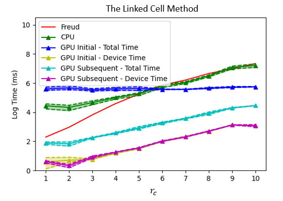
图8 基于Cell List近邻搜索算法的性能表现

alt

图9 基于Hash近邻搜索算法的性能表现

值得注意的是,基于网格的两类方法在较为rc较小时表现不佳,因为此时两类方法均分割了过多的网格(截断半径为1时,网格数量为125000个),对应的处理时间也更长,造成了性能的下降,在计算能力较弱的平台尤为明显。

代码
文本

3. Heatmap对比

我们随后更为详细的比较DP-NBLIST的各算法实现的表现。此处选用场景与之前相同,但粒子数量拓展为[500, 1000, 5000, 10000],比较基准为Freud-AABBTree。

代码
文本
[12]
# heatmap
# ! pip install seaborn
import seaborn as sns

# 绘制相关热力图
def plot_heatmap(data_aabb, data2, title_name):
cmap = plt.cm.RdYlBu

plt.figure(figsize=(6, 4))

# Create the heatmap
ax = sns.heatmap((data_aabb - data2) / data_aabb * 100, cmap=cmap, vmin=-100, vmax=100, annot=True, fmt='.0f')

# Set x-axis ticks and labels
ax.set_xticks(np.arange(len(rc_list)) + 0.5)
ax.set_xticklabels(rc_list)

# Set y-axis ticks and labels
num_particle_list_plot = [f"{num:.0e}" for num in num_particle_list]
ax.set_yticks(np.arange(len(num_particle_list)) + 0.5)
ax.set_yticklabels(num_particle_list_plot, rotation=30)
# Add title and labels
plt.title(title_name, fontsize=12)
plt.xlabel(r'$rc$', fontsize=12)
plt.ylabel(r'$N_p$', fontsize=12)
plt.xticks(fontsize=11)
plt.yticks(fontsize=10)

# Adjust layout to prevent clipping of labels or titles
plt.tight_layout()

# Save the plot as an image file (e.g., PNG)
# plt.savefig(save_name)
plt.show()
plt.close()

run_time_freud_aabb_avg = np.mean(run_time_freud_aabb, axis=2)
# run_time_freud_cellist_avg = np.mean(run_time_freud_cellist, axis=2)

run_time_dp_octree_avg = np.mean(run_time_dp_octree, axis=2)
run_time_dp_celllist_avg = np.mean(run_time_dp_celllist, axis=2)
run_time_dp_hash_avg = np.mean(run_time_dp_hash, axis=2)

plot_heatmap(run_time_freud_aabb_avg, run_time_dp_octree_avg, "Octree CPU - AABB Tree")
plot_heatmap(run_time_freud_aabb_avg, run_time_dp_hash_avg, "Hash CPU - Cell List")
代码
文本

由于Linked Cell算法的表现与Freud-AABBTree近似,我们这里主要给出Octree和Hash算法在更多场景的heatmap结果,包含CPU和GPU架构,以进行进一步分析。此处的heatmap表示各算法实现与Freud-AABBTree算法的性能差异,红色表示相对较慢,蓝色表示相对较快,数值表示相对程度的大小。

alt

图10 基于Octree近邻搜索算法的heatmap

alt

图11 基于Hash近邻搜索算法的heatmap

代码
文本

c. 与DMFF的耦合

此处我们给出一个使用DP_NBLIST辅助DMFF进行水分子模型计算的例子,从准确率和效率两个方面来展示相关结果。

代码
文本
[13]
import imp
import openmm as mm
import openmm.app as app
import openmm.unit as unit
import numpy as np
import sys
from dmff.api import Hamiltonian
import freud

from jax import jit, value_and_grad
import jax.numpy as jnp
import time
# load .so file
nblist = imp.load_dynamic('nblist', '/personal/nblist.cpython-310-x86_64-linux-gnu.so')

代码
文本
[14]
# 基于DP_NBLIST与DMFF耦合的邻居搜索模块
class NeighborListDp:
def __init__(self, alg_type, box, rcut, cov_map, padding=True):
if nblist_module is None:
raise ImportError("nblist not installed.")
self.box = nblist_module.Box([box[0][0], box[1][1], box[2][2]], [90.0, 90.0, 90.0])
self.nb = nblist_module.NeighborList(alg_type)
self.flag = False
self.rcut = rcut
self.capacity_multiplier = None
self.padding = padding
# self.cov_map = np.array(cov_map)
self.cov_map = cov_map
def _do_cov_map(self, pairs):
nbond = self.cov_map[pairs[:, 0], pairs[:, 1]]
pairs = jnp.concatenate([pairs, nbond[:, None]], axis=1)
return pairs

def allocate(self, coords, box=None):
start_time2 = time.time() # 记录开始时间

self._positions = np.array(coords) # cache it
dbox = nblist.Box([box[0][0], box[1][1], box[2][2]], [90.0, 90.0, 90.0]) if box is not None else self.box
self.nb.build(dbox, self._positions, self.rcut)
nlist = self.nb.get_neighbor_pair()

end_time2 = time.time() # 记录结束时间
elapsed_time2 = end_time2 - start_time2 # 计算经过的时间
print(f"neighbor pair: {elapsed_time2} 秒")

msk = (nlist[:, 0] - nlist[:, 1]) < 0
nlist = nlist[msk]
if self.capacity_multiplier is None:
self.capacity_multiplier = int(nlist.shape[0] * 1.3)
if not self.padding:
self._pairs = self._do_cov_map(nlist)
return self._pairs

self.capacity_multiplier = max(self.capacity_multiplier, nlist.shape[0])
padding_width = self.capacity_multiplier - nlist.shape[0]
if padding_width == 0:
self._pairs = self._do_cov_map(nlist)
return self._pairs
elif padding_width > 0:
# padding = np.ones((self.capacity_multiplier - nlist.shape[0], 2), dtype=np.int32) * coords.shape[0]
# nlist = np.vstack((nlist, padding))
self._pairs = self._do_cov_map(nlist)
return self._pairs
else:
raise ValueError("padding width < 0")

def update(self, positions, box=None):
self.allocate(positions, box)

@property
def pairs(self):
return self._pairs

@property
def scaled_pairs(self):
return self._pairs

@property
def positions(self):
return self._positions
代码
文本
[15]
# 基于Freud与DMFF耦合的邻居搜索模块
class NeighborListFreud:
def __init__(self, box, rcut, cov_map, padding=True):
if freud is None:
raise ImportError("Freud not installed.")
self.fbox = freud.box.Box.from_matrix(box)
self.rcut = rcut
self.capacity_multiplier = None
self.padding = padding
self.cov_map = cov_map
def _do_cov_map(self, pairs):
nbond = self.cov_map[pairs[:, 0], pairs[:, 1]]
pairs = jnp.concatenate([pairs, nbond[:, None]], axis=1)
return pairs

def allocate(self, coords, box=None):
start_time2 = time.time() # 记录开始时间
self._positions = coords # cache it

fbox = freud.box.Box.from_matrix(box) if box is not None else self.fbox
aq = freud.locality.AABBQuery(fbox, coords)
res = aq.query(coords, dict(r_max=self.rcut, exclude_ii=True))
nlist = res.toNeighborList()
end_time2 = time.time() # 记录结束时间
elapsed_time2 = end_time2 - start_time2 # 计算经过的时间
print(f"neighbor pair: {elapsed_time2} 秒")

nlist = np.vstack((nlist[:, 0], nlist[:, 1])).T
print(nlist.shape)
nlist = nlist.astype(np.int32)
msk = (nlist[:, 0] - nlist[:, 1]) < 0
nlist = nlist[msk]
print(nlist.shape)
if self.capacity_multiplier is None:
self.capacity_multiplier = int(nlist.shape[0] * 1.3)
if not self.padding:
self._pairs = self._do_cov_map(nlist)
return self._pairs

self.capacity_multiplier = max(self.capacity_multiplier, nlist.shape[0])
padding_width = self.capacity_multiplier - nlist.shape[0]
if padding_width == 0:
self._pairs = self._do_cov_map(nlist)
return self._pairs
elif padding_width > 0:
# padding = np.ones((self.capacity_multiplier - nlist.shape[0], 2), dtype=np.int32) * coords.shape[0]
# nlist = np.vstack((nlist, padding))
self._pairs = self._do_cov_map(nlist)
return self._pairs
else:
raise ValueError("padding width < 0")

def update(self, positions, box=None):
self.allocate(positions, box)

@property
def pairs(self):
return self._pairs

@property
def scaled_pairs(self):
return self._pairs

@property
def positions(self):
return self._positions
代码
文本
[18]
pdb_file = "/share/nblist/EC_box.pdb"
ff_file = '/share/nblist/ffEC.xml'

print("MM Reference Energy:")
start_time = time.time()
pdb = app.PDBFile(pdb_file)
ff = app.ForceField(ff_file)
rc = 1.0
system = ff.createSystem(pdb.topology, nonbondedCutoff=rc*unit.nanometer, nonbondedMethod=app.PME, constraints=None)

h = Hamiltonian(ff_file)
pot = h.createPotential(pdb.topology, nonbondedCutoff=rc*unit.nanometer, nonbondedMethod=app.PME, constraints=None)
efunc = pot.getPotentialFunc()
params = h.getParameters()

pos = jnp.array(pdb.positions._value)
box = jnp.array(pdb.topology.getPeriodicBoxVectors()._value)


print(f"neighbor start")
print(f"cov_map shape: {len(pot.meta['cov_map'])}")
print(f"cov_map shape: {len(pot.meta['cov_map'][0])}")

# 耦合Freud
nbl1 = NeighborListFreud(box, rc, pot.meta['cov_map'])
nbl1.allocate(pos, box)
pairs1 = nbl1.pairs
print(f"pairs shape: {pairs1.shape}")

# 耦合DP_NBLIST
nbl2 = NeighborListDp("Linked_Cell-CPU", box, rc, pot.meta['cov_map'])
nbl2.allocate(pos, box)
pairs2 = nbl2.pairs
print(f"pairs shape: {pairs2.shape}")
MM Reference Energy:
neighbor start
cov_map shape: 10000
neighbor pair: 0.3018181324005127 秒
(3294600, 2)
(1647300, 2)
pairs shape: (1647300, 3)
neighbor pair: 0.2598240375518799 秒
pairs shape: (1647300, 3)
代码
文本

四、规律总结

基于上述结果,我们给出如下使用准则:

a. CPU架构计算

对于CPU架构,当场景较为稀疏,截断半径较小时,建议使用Octree方法;当场景较为稠密,截断半径较大时,建议使用Hash方法;对于介于前两者的场景,也就是目前大部分仿真问题涉及的场景,建议使用Linked Cell方法。

b. GPU架构计算

对于GPU架构,由于各类算法的时间复杂度均为O(n),各实现的表现非常类似,选择任意算法均可满足需求。

c. 异构计算

对于异构计算,规模较小的问题,适于使用CPU架构及对应的使用准则;对于规模较大的问题,则更适于使用GPU架构及对应准则。

(注意上述总结受到平台计算能力的影响,为各类情况的趋势性总结,更为准确的表现需要进行试算才能确定。)

代码
文本
分子动力学
力场
分子动力学力场
已赞1
本文被以下合集收录
AI4S
凝聚态平方
更新于 2024-03-18
32 篇0 人关注
推荐阅读
公开
朱晓彤-第6天-2403-计算材料学原理
2403-计算材料学原理
2403-计算材料学原理
xiaozhu
发布于 2024-03-14
公开
陈宇祥-第6天-2403-计算材料学原理
2403-计算材料学原理
2403-计算材料学原理
yuxiangc22
发布于 2024-03-14