Bohrium
robot
新建

空间站广场

论文
Notebooks
比赛
课程
Apps
我的主页
我的Notebooks
我的论文库
我的足迹

我的工作空间

任务
节点
文件
数据集
镜像
项目
数据库
公开
如何设计一个优雅的机器学习势能函数:以至关重要的等变/协变性、保守性和连续性为例
DPA
PES
Machine Learning
LLM
Material
DPAPES Machine LearningLLMMaterial
zhangd@bjaisi.com
发布于 2023-08-01
推荐镜像 :deepmd-pytorch:cuda12
推荐机型 :c12_m46_1 * NVIDIA GPU B
赞 14
4
4
如何设计一个优雅的机器学习势能函数:以至关重要的等变/协变性、保守性和连续性为例
💭目录
依赖安装
何为“优雅”
等变性
等变性的定义
等变性测试
保守性
保守性的定义
保守性测试
连续性
连续性的定义
连续性测试
总结

如何设计一个优雅的机器学习势能函数:以至关重要的等变/协变性、保守性和连续性为例

©️ Copyright 2023 @ Authors
作者: 张铎 📨
日期:2023-07-30
共享协议:本作品采用知识共享署名-非商业性使用-相同方式共享 4.0 国际许可协议进行许可。
快速开始:点击上方的 开始连接 按钮,选择 deepmd-pytorch:cuda12镜像GPU:c12_m46_1 * NVIDIA GPU B或更高配置机型即可开始。

代码
文本

Open In Bohrium

代码
文本

随着AI for Sicence的发展,基于机器学习的势能函数(Potential Energy Surface,简称PES)模型近年来受到了广泛关注。得益于其在精度上接近第一性原理计算,同时具备与经验力场相媲美的效率,这大大加速了分子动力学应用和研究的推进。其中,应用较为广泛的模型包括Schnet、Dimnet、DeePMD,以及最近的DPA-1、Gemnet、Equiformer等。随着这些模型在特定体系上精度的提升,其结构也变得越来越复杂。然而,在实际应用中,特别是在分子动力学模拟环节,设计模型结构时还需要考虑许多实际因素。

最近,笔者在设计机器学习势能函数时对上述问题有了一些新的体会,希望通过本文向读者分享在面向实际应用场景时,为什么精度并非衡量一个机器学习势能函数优劣的唯一标准,以及在设计一个优雅且适用于下游应用体系的势能函数模型时,需要关注哪些关键因素。

💭目录

代码
文本

依赖安装

代码
文本
已隐藏单元格
Looking in indexes: https://pypi.tuna.tsinghua.edu.cn/simple
Requirement already satisfied: e3nn in /opt/mamba/lib/python3.10/site-packages (0.5.1)
Requirement already satisfied: matplotlib in /opt/mamba/lib/python3.10/site-packages (3.7.2)
Requirement already satisfied: torch>=1.8.0 in /opt/mamba/lib/python3.10/site-packages (from e3nn) (2.0.0+cu118)
Requirement already satisfied: sympy in /opt/mamba/lib/python3.10/site-packages (from e3nn) (1.11.1)
Requirement already satisfied: scipy in /opt/mamba/lib/python3.10/site-packages (from e3nn) (1.10.1)
Requirement already satisfied: opt-einsum-fx>=0.1.4 in /opt/mamba/lib/python3.10/site-packages (from e3nn) (0.1.4)
Requirement already satisfied: packaging>=20.0 in /opt/mamba/lib/python3.10/site-packages (from matplotlib) (23.0)
Requirement already satisfied: contourpy>=1.0.1 in /opt/mamba/lib/python3.10/site-packages (from matplotlib) (1.1.0)
Requirement already satisfied: fonttools>=4.22.0 in /opt/mamba/lib/python3.10/site-packages (from matplotlib) (4.42.0)
Requirement already satisfied: pillow>=6.2.0 in /opt/mamba/lib/python3.10/site-packages (from matplotlib) (10.0.0)
Requirement already satisfied: pyparsing<3.1,>=2.3.1 in /opt/mamba/lib/python3.10/site-packages (from matplotlib) (3.0.9)
Requirement already satisfied: python-dateutil>=2.7 in /opt/mamba/lib/python3.10/site-packages (from matplotlib) (2.8.2)
Requirement already satisfied: kiwisolver>=1.0.1 in /opt/mamba/lib/python3.10/site-packages (from matplotlib) (1.4.4)
Requirement already satisfied: numpy>=1.20 in /opt/mamba/lib/python3.10/site-packages (from matplotlib) (1.24.2)
Requirement already satisfied: cycler>=0.10 in /opt/mamba/lib/python3.10/site-packages (from matplotlib) (0.11.0)
Requirement already satisfied: opt-einsum in /opt/mamba/lib/python3.10/site-packages (from opt-einsum-fx>=0.1.4->e3nn) (3.3.0)
Requirement already satisfied: six>=1.5 in /opt/mamba/lib/python3.10/site-packages (from python-dateutil>=2.7->matplotlib) (1.16.0)
Requirement already satisfied: filelock in /opt/mamba/lib/python3.10/site-packages (from torch>=1.8.0->e3nn) (3.12.0)
Requirement already satisfied: networkx in /opt/mamba/lib/python3.10/site-packages (from torch>=1.8.0->e3nn) (3.0)
Requirement already satisfied: triton==2.0.0 in /opt/mamba/lib/python3.10/site-packages (from torch>=1.8.0->e3nn) (2.0.0)
Requirement already satisfied: typing-extensions in /opt/mamba/lib/python3.10/site-packages (from torch>=1.8.0->e3nn) (4.5.0)
Requirement already satisfied: jinja2 in /opt/mamba/lib/python3.10/site-packages (from torch>=1.8.0->e3nn) (3.1.2)
Requirement already satisfied: cmake in /opt/mamba/lib/python3.10/site-packages (from triton==2.0.0->torch>=1.8.0->e3nn) (3.26.0)
Requirement already satisfied: lit in /opt/mamba/lib/python3.10/site-packages (from triton==2.0.0->torch>=1.8.0->e3nn) (15.0.7)
Requirement already satisfied: mpmath>=0.19 in /opt/mamba/lib/python3.10/site-packages (from sympy->e3nn) (1.3.0)
Requirement already satisfied: MarkupSafe>=2.0 in /opt/mamba/lib/python3.10/site-packages (from jinja2->torch>=1.8.0->e3nn) (2.1.2)
WARNING: Running pip as the 'root' user can result in broken permissions and conflicting behaviour with the system package manager. It is recommended to use a virtual environment instead: https://pip.pypa.io/warnings/venv
代码
文本
已隐藏单元格
代码
文本

何为“优雅”

模型发展一定要为实际下游应用服务

机器学习势能函数模型,顾名思义,是一种通过机器学习建模来拟合并替代传统昂贵的势能函数的方法。其训练数据通常来源于第一性原理计算,例如通过VASP/ABACUS等软件进行DFT计算。数据形式上主要包括原子坐标、元素类型以及计算得到的体系总能量和原子受力等信息。

与计算机视觉和自然语言处理领域相比,在设计机器学习模型时,我们不能简单地增加层数,而需要遵循一定的物理约束(例如各种对称性等)。这一方面是为了提高模型训练的精度,另一方面更重要的是,在使用训练好的模型进行下游应用(如使用LAMMPS进行分子动力学模拟等任务)时,模型需要严格符合各种物理限制。除了最基本的等变/协变性之外,还有一些很重要的约束,如受力的保守性和能量关于坐标的一阶连续性。因为分子动力学模拟本质上是求解牛顿运动方程,如果出现不符合物理约束的情况,模拟过程很容易发生崩溃。当然,机器学习模型乃至于DFT计算,本质上也是对薛定谔方程的近似求解或拟合。从实际应用的角度出发,要近似到什么程度,或者说要坚守哪些必要的物理约束,很大程度上取决于下游任务的需求。然而,在实际操作中,笔者认为以下三个性质是非常重要的且目前还需要始终遵守的约束:等变性,保守性和连续性。在模型设计中,尽管放弃这些约束可能偶尔会提高拟合精度,但在实际应用中,这些性质对于真实应用过程至关重要,甚至能直接决定模型是否具有实际应用价值。

接下来,本教程将尽可能详细地逐一介绍这三个性质,聚焦于如何测试这些性质,并分享一些笔者的个人观点和展望。

代码
文本

等变性

代码
文本

等变性的定义

代码
文本

参考Siyuan Liu同学在"当我们说起神经网络的等变性,我们在谈论什么"这篇notebook中的介绍,笔者将其中的定义适配到机器学习势能函数这个场景这个场景下:

在分子动力学中,有两个很关键的量,分别是整个体系的总能量,以及体系中的原子相互作用产生在原子核上的受力。为了简化我们的表述,在机器学习势能函数这个场景下,模型的输入输出可以被定义为:

其中为原子数量,表示各原子的坐标,为整个体系(材料或分子)的势能,为各原子的受力。 从输入数据格式来看,个三维向量,对应着xyz三个坐标轴上的坐标;由于是整个体系的势能,因此是一个标量一样都是对应到每个原子,且也有xyz三个方向,因此也是个三维向量。即它们的shape为:

在这个场景下,因为模型的输入并不是CV/NLP里面的像素点/单词,而是有实际物理意义的原子坐标,我们必须先验地要求模型的输出关于输入满足一定的对称性,比如能量受力关于输入坐标平移、置换不变性,以及在输入坐标旋转时,能量的不变性和受力的等变/协变性。这里的不变性比较好理解,就是数值不随输入的变化而变化(为了方便表述,受力的序号变化也放在置换不变范围内),而等变性的话,以旋转为例,则是指受力随着坐标的旋转而一起旋转。更为详细的定义可以继续参考上述Siyuan Liu同学的notebook

在实际设计模型的过程中,不变性一般比较好保证(使用相对距离、关于原子序号加和等),所以我们下面也同样只关注受力随着坐标旋转的等变性。

代码
文本

在模型设计上有很多方式可以实现这一等变性,但是在我们实际应用的时候,往往需要显式地让模型保持这一点,而通过数据增强等方式隐式来保持的方式是不严格的,可能会导致实际模拟中的崩溃。

严格的核心思路即是让输出的受力包含旋转矩阵的信息,具体做法有包括向量场/张量场网络、局部坐标系、反向求力等,具体的区别和优劣也在上述notebook中有介绍,这里就不详细展开了。

代码
文本

等变性测试

代码
文本

下面我们来定义一个简单的势能函数模型,并测试其等变性:

代码
文本
[3]
# 随机初始化一个分子里的原子坐标,这里假设只有3个原子;并随机初始化一个旋转矩阵,用它来对坐标进行旋转
natoms = 3
coords = torch.randn(natoms, 3)
rot = o3.rand_matrix()

# 定义网络结构
# 中间embedding层
mlp = nn.Sequential(nn.Linear(1, 128), nn.ReLU(), nn.Linear(128, 128))

# 能量输出层
mlp_energy = nn.Linear(128, 1)

# 受力输出层
mlp_force_1 = nn.Linear(128, 128)
mlp_force_2 = nn.Linear(128, 3, bias=False)
mlp_force = nn.Sequential(mlp_force_1, mlp_force_2)
代码
文本

下面定义三种不同的模型结构,三个模型只有受力的计算方式不同

代码
文本
[4]
# 模型1,通过反向预测模型受力

def model_1(coords):
# shape [natoms_i, 3]
coords.requires_grad_(True)
# shape [natoms_i, natoms_j, 3]
relative_coord = (coords.view(-1, 1, 3) - coords.view(1, -1, 3)) # 计算相对坐标
# shape [natoms_i, natoms_j, 1]
dist = relative_coord.norm(dim=-1).unsqueeze(-1) # 计算距离矩阵
# shape [natoms_i, natoms_j, d]
pair_embed = mlp(dist) # 计算原子间的pair embedding
# shape [natoms_i, d]
atomic_embed = pair_embed.sum(dim=-2)/natoms # 计算均值作为单原子atomic embedding
# shape [natoms_i, 1]
atom_contribution = mlp_energy(atomic_embed).squeeze(-1) # 计算均值作为单原子能量
# shape [1]
energy = atom_contribution.sum(dim=-1) # 取各原子的贡献之和为总能量
# 反向求导预测受力
# shape [natoms_i, 3]
force = -torch.autograd.grad([energy], [coords])[0]
return {'energy': energy, 'force': force}

def test_equivariance(model, model_name):
# 测试能量不变性,若能量不变,则有 model(coords)['energy'] == model(coords @ rot)['energy']
print(f"Energy invariance of {model_name}: ", np.isclose(model(coords)['energy'].detach().numpy(), model(coords @ rot)['energy'].detach().numpy()))
print(f"{model_name}(coords)['energy']: ", model(coords)['energy'].detach().numpy())
print(f"{model_name}(coords @ rot)['energy']: ", model(coords @ rot)['energy'].detach().numpy())
print('\n')

# 测试受力等变性,若受力随旋转等变,则有 model(coords)['force'] @ rot == model(coords @ rot)['force']
print(f"Force equivariance of {model_name}: ", (np.isclose((model(coords)['force'] @ rot).detach().numpy(), model(coords @ rot)['force'].detach().numpy(), rtol=1e-03)).all())
print(f"{model_name}(coords)['force'] @ rot: \n", (model(coords)['force'] @ rot).detach().numpy())
print(f"{model_name}(coords @ rot)['force']: \n", model(coords @ rot)['force'].detach().numpy())
print('\n')

test_equivariance(model_1, 'model_1')
Energy invariance of model_1:  True
model_1(coords)['energy']:  -1.9995141
model_1(coords @ rot)['energy']:  -1.9995142


Force equivariance of model_1:  True
model_1(coords)['force'] @ rot: 
 [[-0.06941875 -0.04426276  0.20484029]
 [-0.1360082   0.18354239 -0.13272315]
 [ 0.20542696 -0.13927963 -0.07211713]]
model_1(coords @ rot)['force']: 
 [[-0.06941876 -0.04426277  0.2048403 ]
 [-0.13600822  0.1835424  -0.13272315]
 [ 0.20542696 -0.13927963 -0.07211715]]


代码
文本
[5]
# 模型2,直接预测受力,但是不考虑等变

def model_2(coords):
# shape [natoms_i, 3]
coords.requires_grad_(False)
# shape [natoms_i, natoms_j, 3]
relative_coord = (coords.view(-1, 1, 3) - coords.view(1, -1, 3)) # 计算相对坐标
# shape [natoms_i, natoms_j, 1]
dist = relative_coord.norm(dim=-1).unsqueeze(-1) # 计算距离矩阵
# shape [natoms_i, natoms_j, d]
pair_embed = mlp(dist) # 计算原子间的pair embedding
# shape [natoms_i, d]
atomic_embed = pair_embed.sum(dim=-2)/natoms # 计算均值作为单原子atomic embedding
# shape [natoms_i, 1]
atom_contribution = mlp_energy(atomic_embed).squeeze(-1) # 计算均值作为单原子能量
# shape [1]
energy = atom_contribution.sum(dim=-1) # 取各原子的贡献之和为总能量
# 直接通过mlp预测受力
# shape [natoms_i, 3]
force = mlp_force(atomic_embed)
return {'energy': energy, 'force': force}


test_equivariance(model_2, 'model_2')
Energy invariance of model_2:  True
model_2(coords)['energy']:  -1.9995141
model_2(coords @ rot)['energy']:  -1.9995142


Force equivariance of model_2:  False
model_2(coords)['force'] @ rot: 
 [[-0.09841716 -0.00249557  0.10106925]
 [-0.10416244 -0.00117455  0.11785105]
 [-0.10268676 -0.0014452   0.11389805]]
model_2(coords @ rot)['force']: 
 [[0.01968813 0.12475397 0.0628965 ]
 [0.01439494 0.14055493 0.06911699]
 [0.01553482 0.13676846 0.06762004]]


代码
文本
[6]
# 模型3,直接预测受力,但是乘以相对坐标,考虑了旋转矩阵

def model_3(coords):
# shape [natoms_i, 3]
coords.requires_grad_(False)
# shape [natoms_i, natoms_j, 3]
relative_coord = (coords.view(-1, 1, 3) - coords.view(1, -1, 3)) # 计算相对坐标
# shape [natoms_i, natoms_j, 1]
dist = relative_coord.norm(dim=-1).unsqueeze(-1) # 计算距离矩阵
# shape [natoms_i, natoms_j, d]
pair_embed = mlp(dist) # 计算原子间的pair embedding
# shape [natoms_i, d]
atomic_embed = pair_embed.sum(dim=-2)/natoms # 计算均值作为单原子atomic embedding
# shape [natoms_i, 1]
atom_contribution = mlp_energy(atomic_embed).squeeze(-1) # 计算均值作为单原子能量
# shape [1]
energy = atom_contribution.sum(dim=-1) # 取各原子的贡献之和为总能量
# 直接预测受力,但是乘以相对坐标,考虑了旋转矩阵
# shape [natoms_i, d, 3]
rot_mat = torch.matmul(pair_embed.transpose(1,2), relative_coord)
# shape [natoms_i, 3]
force = torch.matmul(mlp_force_1(atomic_embed).reshape(natoms, 1, 128), rot_mat).reshape(natoms, 3)
return {'energy': energy, 'force': force}


test_equivariance(model_3, 'model_3')
Energy invariance of model_3:  True
model_3(coords)['energy']:  -1.9995141
model_3(coords @ rot)['energy']:  -1.9995142


Force equivariance of model_3:  True
model_3(coords)['force'] @ rot: 
 [[-2.2367618 -1.9168309  7.569722 ]
 [-8.414907  10.547373  -6.614018 ]
 [10.645403  -7.926773  -2.3357892]]
model_3(coords @ rot)['force']: 
 [[-2.2367616 -1.9168317  7.569721 ]
 [-8.414906  10.547375  -6.6140184]
 [10.645401  -7.9267697 -2.33579  ]]


代码
文本

通过上述测试可以看到:

model_1通过反向求力,即 来保证了受力的等变性;

model_2直接预测受力,但是并没有对受力等变性做任何假设,即使最后输出层不加bias,也不能保证受力的等变性;

model_3通过直接预测受力的同时,在输出的最后乘以了和坐标相关的旋转矩阵rot_mat,于是也保持了受力的等变性。

代码
文本

保守性

代码
文本

保守性的定义

代码
文本

在实际应用中,特别是在进行真实体系模拟时(例如在LAMMPS中使用机器学习势能函数进行分子动力学模拟),我们需要更严格的约束。本部分将重点介绍保守性,即受力必须严格为能量关于输入坐标的负梯度

这与上一部分中model_1的反向求力方法相对应。这是因为在分子动力学模拟中,受力的保守性是一个基本的假设,受力的保守可以确保能量守恒、轨迹可逆性、减少误差累积等。具体来说:

  1. 能量守恒:在保守力系统中,系统的总能量(动能与势能之和)在模拟过程中将保持恒定,这是分子动力学模拟的基本要求;

  2. 轨迹可逆性:在保守力系统中,分子动力学模拟轨迹具有时间可逆性。这意味着,如果在某个时刻将所有粒子的速度反转,系统将沿着原来的轨迹返回到初始状态。这对于理解微观尺度下物质行为和分子间相互作用机制具有重要意义;

  3. 减少误差累积:保守力在计算过程中不会引入额外误差,有助于确保模拟的准确性,而非保守力可能导致误差逐渐累积,从而影响模拟结果的可靠性。

代码
文本

保守性测试

代码
文本

下面我们通过对数值导数和解析导数一致性的测试,来验证model_1和model_3的受力保守性。

代码
文本
[7]
# 受力保守性测试
def test_conserv(model, model_name):
model_pred = model(coords)
energy_output = model_pred['energy']
force_output = model_pred['force']
numerical_force = torch.zeros_like(force_output)
epsilon = 1e-3
for atom_i in range(natoms):
for axis in range(3):
coords_tmp = coords.clone()
coords_tmp[atom_i][axis] += epsilon
energy_tmp = model(coords_tmp)['energy']
numerical_force[atom_i][axis] = -(energy_tmp - energy_output)/epsilon
# 测试受力保守性,若受力保守,则有 force_output == numerical_force
print(f"Force conservativeness of {model_name}: ", np.isclose(force_output.detach().numpy(), numerical_force.detach().numpy(), atol=1e-02).all())
print(f"force output of {model_name}: \n", force_output)
print(f"numerical force of {model_name}: \n", numerical_force)

# 测试model_1受力的保守性
test_conserv(model_1, 'model_1')
Force conservativeness of model_1:  True
force output of model_1: 
 tensor([[-0.0411,  0.2154,  0.0251],
        [ 0.0995, -0.1255,  0.2101],
        [-0.0584, -0.0899, -0.2352]])
numerical force of model_1: 
 tensor([[-0.0409,  0.2158,  0.0253],
        [ 0.0997, -0.1254,  0.2103],
        [-0.0582, -0.0896, -0.2348]], grad_fn=<CopySlices>)
代码
文本
[8]
# 测试model_3受力的保守性
test_conserv(model_3, 'model_3')
Force conservativeness of model_3:  False
force output of model_3: 
 tensor([[ -1.6521,   7.9362,   0.5158],
        [  5.6194,  -6.1282,  12.5168],
        [ -3.4994,  -3.2226, -12.6089]], grad_fn=<ReshapeAliasBackward0>)
numerical force of model_3: 
 tensor([[-0.0409,  0.2158,  0.0253],
        [ 0.0997, -0.1254,  0.2103],
        [-0.0582, -0.0896, -0.2348]], grad_fn=<CopySlices>)
代码
文本

可以看到,model_1通过直接在模型中进行反向求导,严格保证了受力等于能量关于输入坐标的负梯度,从而确保了受力的保守性。

而对于model_3,虽然其确保了受力的协变性,但由于没有显式地保证受力等于能量关于输入坐标的负梯度,因此其受力是不保守的。

在实际应用中,这两种方式各有优劣

反向求导预测受力的model_1,虽然其保守性有保证,但是由于在模型训练、推理时都要多反传一次,导致其计算效率稍低,且占用显存较大;

直接预测受力的model_3,计算效率高,且在某些数据驱动的体系上拟合精度会更好一些,但是无法用于分子动力学模拟。

代码
文本

连续性

代码
文本

连续性的定义

代码
文本

在实际应用中,除了之前讨论较多的两个物理约束之外,笔者最近对连续性这一容易被忽视的性质有了更深刻的认识。在许多材料体系中,有时仅仅因为在一个细小的部分忽略了连续性,可能会导致巨大的影响。

以最近的一些具体实践为例,在某个环节没有充分考虑连续性,在半导体或二维材料等体系上的训练效果可能会出现数量级的差异。下图展示了两个实验,蓝色线代表保持连续性,红色线代表不保持连续性,分别展示了它们在能量和受力的训练、测试误差随训练步数的变化:

从图中可以看出,不保持连续性的红色线误差相较于蓝色线有数量级的差距。

那么我们接下来着重讨论下连续性的定义和测试方式。

代码
文本

首先,连续性本身的定义很简单,一阶的连续性用语言表述即在模型输入发生细微变化的时候,模型的输出不能发生剧烈变化

这一点看似很简单,但是在实际应用导向的模型设计中,往往被忽视,从而会导致一系列的问题,比如在LAMMPS模拟的时候突然发生能量跳变,使得最小化线搜索等搜不到正确的步长,直接导致模拟崩溃等。

我们通过下面的连续性测试来更直观体会连续性问题。

代码
文本

连续性测试

代码
文本

大家可能会注意到,在面对只有三个原子的系统时,很难将其与连续性联系起来。这是因为整个系统规模过小,而模型设计本身是一个全局模型。也就是说,对于每个中心原子,我们需要考虑与所有其他原子的相互作用,这样很难体现出连续性的问题。

然而,在实际应用中,我们的模拟系统往往包含成千上万个原子,模拟过程中的原子甚至可能分布在多台不同的机器上。在这种情况下,全局模型所带来的计算代价是完全无法接受的。因此,在实践中,我们通常会采用截断半径的方法来实现一个局部模型

具体来说,我们会选择一个合理的截断半径 ,以每个原子为球心,只考虑半径为 的球内部的原子作为该原子的邻居,球外的相互作用则不予考虑。这也是为什么机器学习势能函数能够进行上亿原子的分子动力学模拟的基本假设。

代码
文本

在这种情况下,模型的连续性变得至关重要。从一个中心原子的视角来看,我们可以设想,当一个相邻原子在临界距离附近发生变化时,即在半径为的球内进出时,模型的输出需要经过精心设计以避免发生剧烈变化。

代码
文本

为了更直观地看到上述影响,我们把上述的model_1更改为局部模型:(model_3的能量和model_1完全一致,故省略)

代码
文本
[9]
natoms = 4
coords_smth_test = torch.tensor([0., 0., 0.,
4., 0., 0.,
0., 4., 0.,
0., 0., 4.,]).view([natoms, 3])


# 模型1局部版,通过反向预测模型受力

def model_1_local(coords, rcut=4.0):
# shape [natoms_i, 3]
coords.requires_grad_(True)
# shape [natoms_i, natoms_j, 3]
relative_coord = (coords.view(-1, 1, 3) - coords.view(1, -1, 3)) # 计算相对坐标
# shape [natoms_i, natoms_j, 1]
dist = relative_coord.norm(dim=-1).unsqueeze(-1) # 计算距离矩阵
# shape [natoms_i, natoms_j, 1]
neighbor_mask = (dist <= rcut) & (dist > 0) # 计算局部的mask,排除距离自己超过rcut的邻居原子以及自己本身
# shape [natoms_i, natoms_j, d]
pair_embed = mlp(dist) # 计算原子间的pair embedding
# shape [natoms_i, natoms_j, d]
pair_embed_masked = pair_embed*neighbor_mask
# shape [natoms_i, d]
atomic_embed = pair_embed_masked.sum(dim=-2)/(natoms-1) # 计算均值作为单原子atomic embedding
# shape [natoms_i, 1]
atom_contribution = mlp_energy(atomic_embed).squeeze(-1) # 计算均值作为单原子能量
# shape [1]
energy = atom_contribution.sum(dim=-1) # 取各原子的贡献之和为总能量
# 反向求导预测受力
# shape [natoms_i, 3]
force = -torch.autograd.grad([energy], [coords])[0]
return {'energy': energy, 'force': force}
代码
文本

接下来,通过对输入坐标在周围进行扰动,观察输出能量的变化情况,从而测试其连续性:

代码
文本
[11]
def test_smooth(model, model_name, epsilon=1e-4, verbose=True):
coord0 = coords_smth_test.clone()
coord1 = coords_smth_test.clone()
coord1[1][0] += epsilon
coord2 = coords_smth_test.clone()
coord2[2][1] += epsilon
coord3 = coords_smth_test.clone()
coord3[1][0] += epsilon
coord3[2][1] += epsilon
model_pred_0 = model(coord0)['energy'].detach().numpy()
model_pred_1 = model(coord1)['energy'].detach().numpy()
model_pred_2 = model(coord2)['energy'].detach().numpy()
model_pred_3 = model(coord3)['energy'].detach().numpy()
# 测试能量连续性,若能量连续,则有 model_pred_0 == model_pred_1 == model_pred_2 == model_pred_3
smooth = np.isclose(model_pred_0, model_pred_1) and np.isclose(model_pred_0, model_pred_2) and np.isclose(model_pred_0, model_pred_3)
if verbose:
print(f"Energy smoothness of {model_name}: ", smooth)
print(f"base energy of {model_name}:", model_pred_0)
print(f"small perturbed 1 of {model_name}:", model_pred_1)
print(f"small perturbed 2 of {model_name}:", model_pred_2)
print(f"small perturbed 3 of {model_name}:", model_pred_3)
return float(model_pred_1)


def plot_smooth(model, model_name):
out_x = []
out_y = []
for i in range(-10, 10):
out_x.append(1e-4 * i)
out_y.append(test_smooth(model, model_name, epsilon=1e-4 * i, verbose=False))
fig, ax = plt.subplots(1, 1, figsize=(10, 6))
ax.set_xlim((-1e-3, 1e-3))
ax.set_ylim((-10, 10))
ax.plot(out_x, out_y, marker='.',color='r')
ax.set_xlabel("Perturbation near $r_{cut}$: $\AA$")
ax.set_ylabel("Predicted energy: eV")
ax.set_title(f"Energy smooth test on {model_name}")

test_smooth(model_1_local, 'model_1_local')
plot_smooth(model_1_local, 'model_1_local')
Energy smoothness of model_1_local:  False
base energy of model_1_local: -2.219089
small perturbed 1 of model_1_local: -1.5245751
small perturbed 2 of model_1_local: -1.5245751
small perturbed 3 of model_1_local: -0.8300612
代码
文本

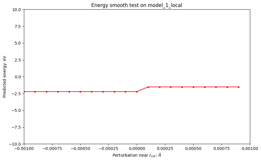
可以看到,model_1_local并不具有连续性,在附近进行扰动(< 1e-3)时,输出可能会发生巨变。

根本原因是model_1_local里面对pair_embed_masked的计算:

pair_embed_masked = pair_embed * neighbor_mask
atomic_embed = pair_embed_masked.sum(dim=-2)/natoms

这里会导致atomic_embed在neighbor_mask发生突变的时候也发生突变,导致最终输出不连续。

代码
文本

在实际应用中,这种不连续往往会造成很大问题。针对这个问题,笔者这里提出几个可能的方案:

  1. 由于这里的atomic_embed本质是对pair_embed的平均,是否可以改为masked mean来解决?即把分母(natoms-1)换为里面真实的邻居数;
  2. 本质上是要对进出的时候的增减量进行连续化,能否变为加权平均,并使得权重和距离相关?
代码
文本

接下来我们分别对上述两种方式进行验证。

代码
文本

首先试试将atomic_embed改为masked mean:

代码
文本
[12]
# 模型1局部版,通过反向预测模型受力,增加masked_mean

def model_1_local_masked_mean(coords, rcut=4.0):
# shape [natoms_i, 3]
coords.requires_grad_(True)
# shape [natoms_i, natoms_j, 3]
relative_coord = (coords.view(-1, 1, 3) - coords.view(1, -1, 3)) # 计算相对坐标
# shape [natoms_i, natoms_j, 1]
dist = relative_coord.norm(dim=-1).unsqueeze(-1) # 计算距离矩阵
# shape [natoms_i, natoms_j, 1]
neighbor_mask = (dist <= rcut) & (dist > 0) # 计算局部的mask,排除距离自己超过rcut的邻居原子以及自己本身
neighbor_mask_num = neighbor_mask.squeeze(-1).sum(-1).unsqueeze(-1) # 计算mask的真实邻居数
# shape [natoms_i, natoms_j, d]
pair_embed = mlp(dist) # 计算原子间的pair embedding
# shape [natoms_i, natoms_j, d]
pair_embed_masked = pair_embed*neighbor_mask
# shape [natoms_i, d]
atomic_embed = pair_embed_masked.sum(dim=-2)/(neighbor_mask_num + 1e-6) # 计算均值作为单原子atomic embedding
# shape [natoms_i, 1]
atom_contribution = mlp_energy(atomic_embed).squeeze(-1) # 计算均值作为单原子能量
# shape [1]
energy = atom_contribution.sum(dim=-1) # 取各原子的贡献之和为总能量
# 反向求导预测受力
# shape [natoms_i, 3]
force = -torch.autograd.grad([energy], [coords])[0]
return {'energy': energy, 'force': force}

test_smooth(model_1_local_masked_mean, 'model_1_local_masked_mean')
plot_smooth(model_1_local_masked_mean, 'model_1_local_masked_mean')
Energy smoothness of model_1_local_masked_mean:  False
base energy of model_1_local_masked_mean: -4.302627
small perturbed 1 of model_1_local_masked_mean: -3.260857
small perturbed 2 of model_1_local_masked_mean: -3.2608573
small perturbed 3 of model_1_local_masked_mean: -2.219087
代码
文本

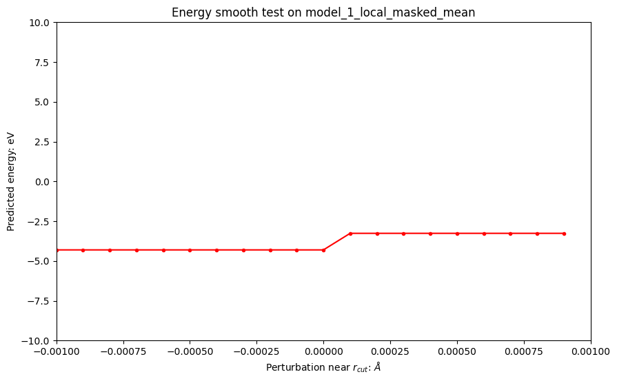
我们可以看到,尽管我们采用了masked_mean方法,但仍无法确保结果的连续性。这是因为虽然分母是真实的邻居数量,但分子中的突变仍然存在。

需要特别指出的是,在许多网络的attention操作中,都采用了masked_mean方法。虽然这种方法在一定程度上能够减缓结果不连续性的问题,但仍无法完全解决。

代码
文本

接下来我们尝试一下连续化的加权平均。

首先定义连续化的权重,和DeePMD-kit/DPA-1中使用的一致

代码
文本

其中时原子距离,为稍小于的连续截断半径,可视化出关于的图像为:

代码
文本
[13]
# 定义连续化的权重,和DeePMD-kit/DPA-1中使用的一致
def switch_function(distance, rmin=0.5, rmax=4.0):
"""Compute smooth weight for descriptor elements."""
min_mask = distance <= rmin
max_mask = distance >= rmax
mid_mask = torch.logical_not(torch.logical_or(min_mask, max_mask))
uu = (distance - rmin) / (rmax - rmin)
vv = uu * uu * uu * (-6 * uu * uu + 15 * uu - 10) + 1
return (1/(distance+1e-6)) * (vv * mid_mask + min_mask)


x_dist = []
y_sw = []
for i in range(100):
dist_tmp = float(i)/80 * 4.0
x_dist.append(dist_tmp)
y_sw.append(switch_function(torch.tensor(dist_tmp)))
fig, ax = plt.subplots(1, 1, figsize=(10, 6))
ax.plot(x_dist, y_sw, marker='.',color='r')
ax.set_ylim((0, 2))
ax.set_xlabel("Perturbation near $r_{cut}$: $\AA$")
ax.set_ylabel("Predicted energy: eV")
ax.set_title(f"Energy smooth test on")
Text(0.5, 1.0, 'Energy smooth test on')
代码
文本
[14]
# 模型1局部版,通过反向预测模型受力,增加连续化的加权平均:

def model_1_local_smooth_average(coords, rcut=4.0):
# shape [natoms_i, 3]
coords.requires_grad_(True)
# shape [natoms_i, natoms_j, 3]
relative_coord = (coords.view(-1, 1, 3) - coords.view(1, -1, 3)) # 计算相对坐标
# shape [natoms_i, natoms_j, 1]
dist = relative_coord.norm(dim=-1).unsqueeze(-1) # 计算距离矩阵
# shape [natoms_i, natoms_j, 1]
neighbor_mask = (dist <= rcut) & (dist > 0) # 计算局部的mask,排除距离自己超过rcut的邻居原子以及自己本身
# shape [natoms_i, natoms_j, d]
pair_embed = mlp(dist) # 计算原子间的pair embedding
# shape [natoms_i, natoms_j, d]
pair_embed_masked = pair_embed*neighbor_mask
pair_embed_masked = pair_embed_masked*switch_function(dist)
# print(switch_function(dist))
# shape [natoms_i, d]
# print(switch_function(dist).shape)
atomic_embed = (pair_embed_masked).sum(dim=-2)/(natoms-1) # 计算均值作为单原子atomic embedding
# shape [natoms_i, 1]
atom_contribution = mlp_energy(atomic_embed).squeeze(-1) # 计算均值作为单原子能量
# shape [1]
energy = atom_contribution.sum(dim=-1) # 取各原子的贡献之和为总能量
# 反向求导预测受力
# shape [natoms_i, 3]
force = -torch.autograd.grad([energy], [coords])[0]
return {'energy': energy, 'force': force}

test_smooth(model_1_local_smooth_average, 'model_1_local_smooth_average')
plot_smooth(model_1_local_smooth_average, 'model_1_local_smooth_average')
Energy smoothness of model_1_local_smooth_average:  True
base energy of model_1_local_smooth_average: -0.13554725
small perturbed 1 of model_1_local_smooth_average: -0.13554725
small perturbed 2 of model_1_local_smooth_average: -0.13554725
small perturbed 3 of model_1_local_smooth_average: -0.13554725
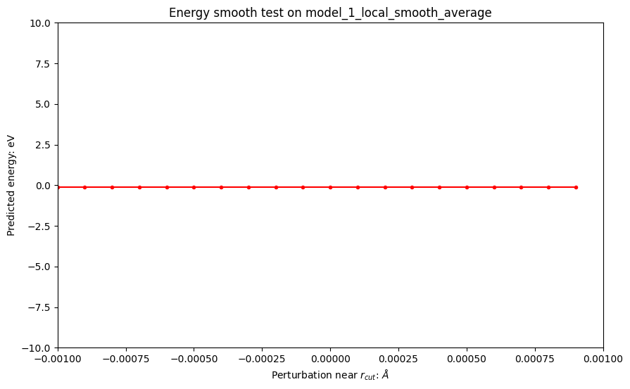
代码
文本

可以看到,能量的连续性得到了保证。

在实际应用中,并不是直接乘以这个连续性权重,但是核心思路和这个类似,具体可以参考DPA-1 paper中的处理;同时,在包含attention操作的模型中,对attention weights也需要有类似的处理来保证连续性。

思考:在其他模型中,也有对相关连续性的处理,比如Gemnet中使用了连续的neighbor list,但是仍然会在边界上存在一些问题;也有一些模型使用了Gaussian kernel来替代上述的switch_function,虽然在边界上已经很接近0,但也并不是完全的连续性。

代码
文本

总结

代码
文本

在本篇notebook中,我们探讨了在实际应用场景中设计机器学习势能函数时需要关注的问题。我们从等变性、保守性和连续性三个关键性质进行了讨论,希望能为读者提供一些参考。在设计网络时,虽然有时候放弃这些物理约束可能会带来更高的精度,但在具体应用过程中,我们还需权衡是否值得用这些精度提升来牺牲模型的实用性。

代码
文本
DPA
PES
Machine Learning
LLM
Material
DPAPES Machine LearningLLMMaterial
已赞14
本文被以下合集收录
machine learning
hjchen
更新于 2024-02-26
16 篇7 人关注
DeepMD-kit与lammps
bohrb27761
更新于 2024-06-19
13 篇3 人关注
推荐阅读
公开
如何设计一个优雅的机器学习势能函数:以至关重要的等变/协变性、保守性和连续性为例
DPAPES Machine LearningLLMMaterial
CyrusZHOU
发布于 2024-04-01
1 赞
公开
浅谈STEM图像|机器学习助力材料图像表征
Machine LearningAI4SSTEM
hongyanhui
发布于 2023-07-24
15 赞21 转存文件4 评论
评论
 # 模型1,通过反向预测模型受力 de...

Atom Hacker

02-20 22:52
这里还有下面的atom_contribution的shape都是[natoms_i]吧。
评论