


Random Signals
🏃🏻 Getting Started Guide
This document can be executed directly on the Bohrium Notebook. To begin, click the Connect button located at the top of the interface, then select the digital-signal-processing:Digital-Signal-Processing-Lecture Image and choose your desired machine configuration to proceed.
📖 Source
This Notebook is from a famous Signal Processing Lecture. The notebooks constitute the lecture notes to the masters course Digital Signal Processing read by Sascha Spors, Institute of Communications Engineering, Universität Rostock.
This jupyter notebook is part of a collection of notebooks on various topics of Digital Signal Processing. Please direct questions and suggestions to Sascha.Spors@uni-rostock.de.
Introduction
Random signals are signals whose values are not (or only to a limited extend) predictable. Frequently used alternative terms are
- stochastic signals
- non-deterministic signals
Random signals play an important role in various fields of signal processing and communications. This is due to the fact that only random signals carry information. A signal which is observed by a receiver has to be unknown to some degree in order to represent novel information.
Random signals are often classified as useful/desired and disturbing/interfering signals. For instance
- useful signals: data, speech, music, images, ...
- disturbing signals: thermal noise at a resistor, amplifier noise, quantization noise, cosmic microwave background...
Practical signals are frequently modeled as a combination of useful signals and additive noise.
As the values of a random signal cannot be foreseen, the properties of random signals are described by the their statistical characteristics. One measure is for instance the average value of a random signal.
Example - Random Signals
The following audio examples illustrate the characteristics of some deterministic and random signals. Lower the volume of your headphones or loudspeakers before playing back the examples.
Cosine signal
Noise
Cosine signal superpositioned by noise
Speech signal
Speech signal superpositioned by noise
Excercise
- Which example can be considered as deterministic, random signal or combination of both?
Solution: The cosine signal is the only deterministic signal. Noise and speech are random signals, as their samples can not (or only to a limited extend) be predicted from previous samples. The superposition of the cosine and noise signals is a combination of a deterministic and a random signal.
Processing of Random Signals
In contrary to the assumption of deterministic signals in traditional signal processing, statistical signal processing treats signals explicitly as random signals. Two prominent application examples involving random signals are:
Measurement of physical quantities
The measurement of physical quantities is often subject to additive noise and distortions. The additive noise models e.g. the sensor noise. The distortions, by e.g. the transmission properties of an amplifier, may be modeled by a system.

denotes an arbitrary (not necessarily LTI) system. The aim of statistical signal processing is to estimate the physical quantity from the observed sensor data, given some knowledge on the disturbing system and the statistical properties of the noise.
Communication channel
In communications engineering a message is sent over a channel that distorts the signal by e.g. multipath propagation. Additive noise is present at the receiver due to background and amplifier noise.

The aim of statistical signal processing is to estimate the sent message from the received message, given some knowledge on the disturbing system and the statistical properties of the noise.
Random Processes
A random process is a stochastic process which generates an ensemble of random signals. A random process
- provides a mathematical model for an ensemble of random signals and
- generates different sample functions with specific common properties.
It is important to differentiate between an
- ensemble: collection of all possible signals of a random process and an
- sample function: one specific random signal.
An example for a random process is speech produced by humans. Here the ensemble is composed from the speech signals produced by all humans on earth, one particular speech signal produced by one person at a specific time is a sample function.
Example - Sample functions of a random process
The following example shows sample functions of a continuous amplitude real-valued random process. All sample functions have the same properties with respect to certain statistical measures.
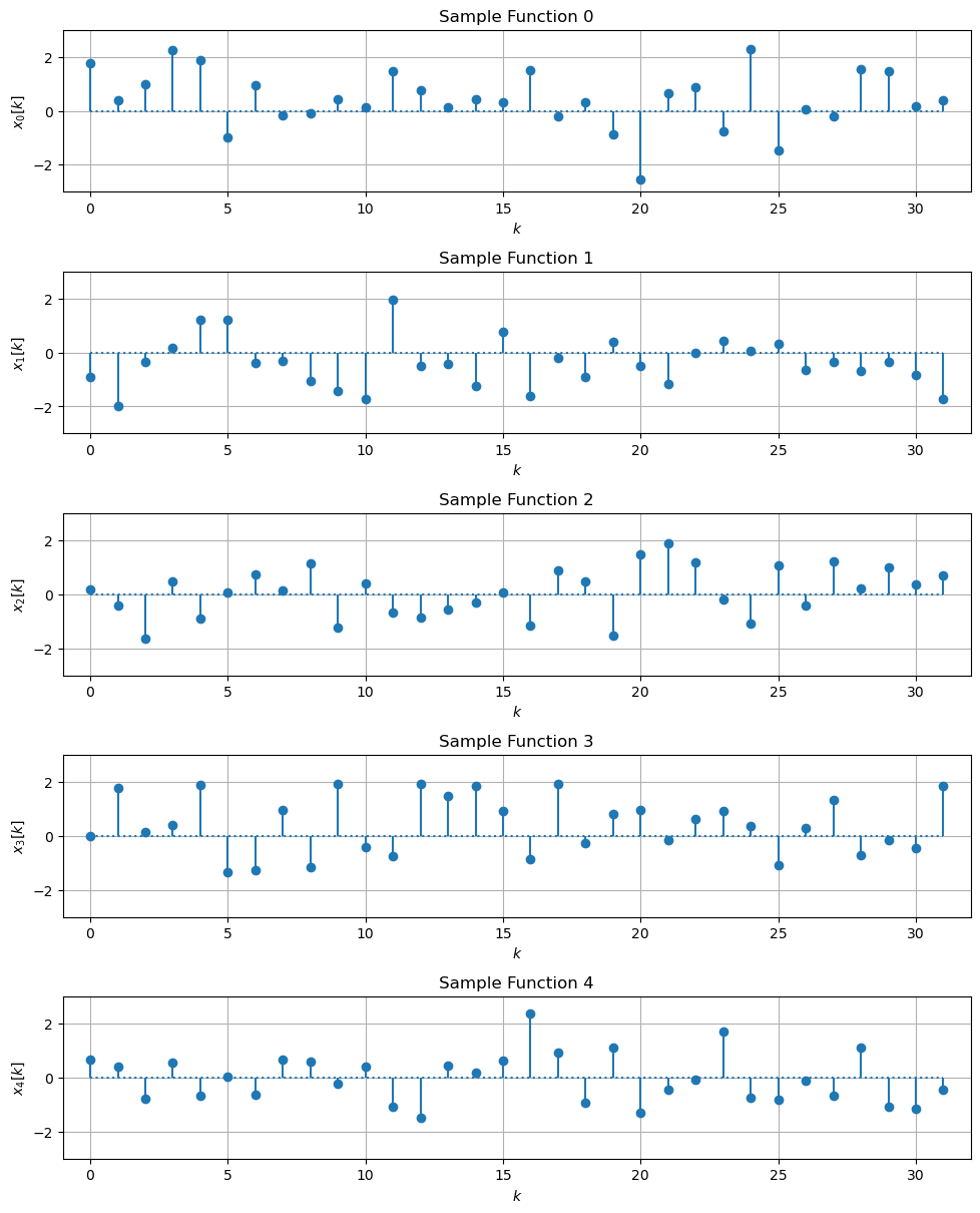
Exercise
- What is different, what is common between the sample functions?
Solution: You may have observed that the amplitude values of the individual sample functions differ for a fixed time instant . However, the sample functions seem to share some common properties. For instance, positive and negative values seem to occur with approximately the same probability. Furthermore, positive and negative values seem to be aligned around zero.
Properties of Random Processes and Random Signals
It was already argued above, that it is not meaningful to describe a random signal by the amplitude values of a particular sample function. Instead, random signals are characterized by specific statistical measures. In statistical signal processing it is common to use
- amplitude distributions and
- ensemble averages/moments
for this purpose. These measures will be introduced in the following.
Copyright
This notebook is provided as Open Educational Resource. Feel free to use the notebook for your own purposes. The text is licensed under Creative Commons Attribution 4.0, the code of the IPython examples under the MIT license. Please attribute the work as follows: Sascha Spors, Digital Signal Processing - Lecture notes featuring computational examples.