Bohrium
robot
新建

空间站广场

论文
Notebooks
比赛
课程
Apps
我的主页
我的Notebooks
我的论文库
我的足迹

我的工作空间

任务
节点
文件
数据集
镜像
项目
数据库
公开
pyGenomeTracks:多维基因组数据的高质量可视化
中文
生物信息学
基因组
可视化
中文生物信息学基因组可视化
Judy Lin
发布于 2023-08-07
推荐镜像 :ubuntu22-py310-r43-gpu-0803n:BioPlot
推荐机型 :c2_m4_cpu
赞 2
3
pyGenomeTracks:多维基因组数据的高质量可视化
Basic Examples
Examples with bed and gtf
Examples with 4C-seq
Examples with peaks
Example with horizontal lines
Examples with Epilogos
Examples with multiple options
Examples with multiple options for bigwig tracks
Examples with Hi-C data
Log transform and Operation Examples
References

pyGenomeTracks:多维基因组数据的高质量可视化

Open In Bohrium

嘿!你是否曾经为了分析和可视化基因组数据而感到头疼?面对大量的复杂信息,你是否感觉有点不知所措?别担心,我来帮你解决这个问题!

让我向你介绍pyGenomeTracks(PGT),这是一个令人兴奋的新软件,它可以帮助你在基因组数据的海洋中找到自己的方向。你可能会问,这个软件有什么特别之处?好问题!

首先,我们都知道基因组数据分析涉及许多复杂的步骤,而PGT正是为了解决这些挑战而诞生的。它可以轻松处理大规模数据,帮助你在全基因组水平上进行快速而高效的分析和总结。对于研究人员来说,这意味着更多的时间和精力可以用于深入挖掘数据中隐藏的宝藏。

其次,PGT还提供了强大的可视化功能,可以让你在基因组上绘制各种数据轨迹。无论是基因注释、基因表达还是染色质信号和互作信息,它都能轻松应对。最重要的是,它可以将这些信息融合到一个统一的图像中,让你一目了然。

PGT的使用也非常简单!你只需要准备一个配置文件,指定你想要绘制的轨迹和数据源,然后运行一个简单的命令行,就能生成高质量的图像。不用再为复杂的数据处理过程和图像生成而烦恼了!

如果你喜欢图形界面,也别担心!PGT还提供了图形化界面,让你可以更直观地进行操作。

所以,如果你是一个对基因组数据感兴趣的研究者或生物信息学家,PGT绝对是你不可或缺的利器!它将帮助你轻松解决数据分析和可视化难题,让你在基因组探索的旅程中事半功倍!

让我们一起走进pyGenomeTracks的神奇世界,开启一段令人激动的基因组探索之旅吧!

📖 上手指南
共享协议:本作品采用知识共享署名-非商业性使用-相同方式共享 4.0 国际许可协议进行许可。
快速开始:本文档可在 Bohrium Notebook 上直接运行。点击上方的 开始连接 按钮,选择 ubuntu22-py310-r43-gpu-0803n:plot镜像R kernel和任意节点即可开始。

代码
文本
[1]
! cd /pyGenomeTracks/
代码
文本

Basic Examples

A minimal example of a configuration file with a single bigwig track looks like this:

代码
文本
[7]
#[bigwig file test]
file = "bigwig2_X_2.5e6_3.5e6.bw"
# height of the track in cm (optional value)
height = 4
title = "bigwig2"
min_value = 0
max_value = 30
代码
文本
[9]
! pyGenomeTracks --tracks ./examples/bigwig_track.ini --region X:2,500,000-3,000,000 -o ./examples/bigwig.png
usage: pyGenomeTracks --tracks tracks.ini --region chr1:1000000-4000000 -o image.png
pyGenomeTracks: error: argument --tracks: can't open './examples/bigwig_track.ini': [Errno 2] No such file or directory: './examples/bigwig_track.ini'
代码
文本

figure5

代码
文本

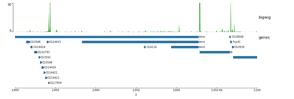
Now, let’s add the genomic location and some genes:
代码
文本
[ ]
[bigwig file test]
file = bigwig.bw
# height of the track in cm (optional value)
height = 4
title = bigwig
min_value = 0
max_value = 30

[spacer]
# this simply adds an small space between the two tracks.

[genes]
file = genes.bed.gz
height = 7
title = genes
fontsize = 10
file_type = bed
gene_rows = 10

[x-axis]
fontsize=10
代码
文本
[ ]
$ pyGenomeTracks --tracks bigwig_with_genes.ini --region X:2,800,000-3,100,000 -o bigwig_with_genes.png
代码
文本

figure6

代码
文本

Now, we will add some vertical lines across all tracks. The vertical lines should be in a bed format.

代码
文本
[ ]
[bigwig file test]
file = bigwig.bw
# height of the track in cm (optional value)
height = 4
title = bigwig
min_value = 0
max_value = 30

[spacer]
# this simply adds an small space between the two tracks.

[genes]
file = genes.bed.gz
height = 7
title = genes
fontsize = 10
file_type = bed
gene_rows = 10

[x-axis]
fontsize=10

[vlines]
file = domains.bed
type = vlines
代码
文本
[ ]
! pyGenomeTracks --tracks bigwig_with_genes_and_vlines.ini --region X:2,800,000-3,100,000 -o bigwig_with_genes_and_vlines.png
代码
文本

figure7

代码
文本

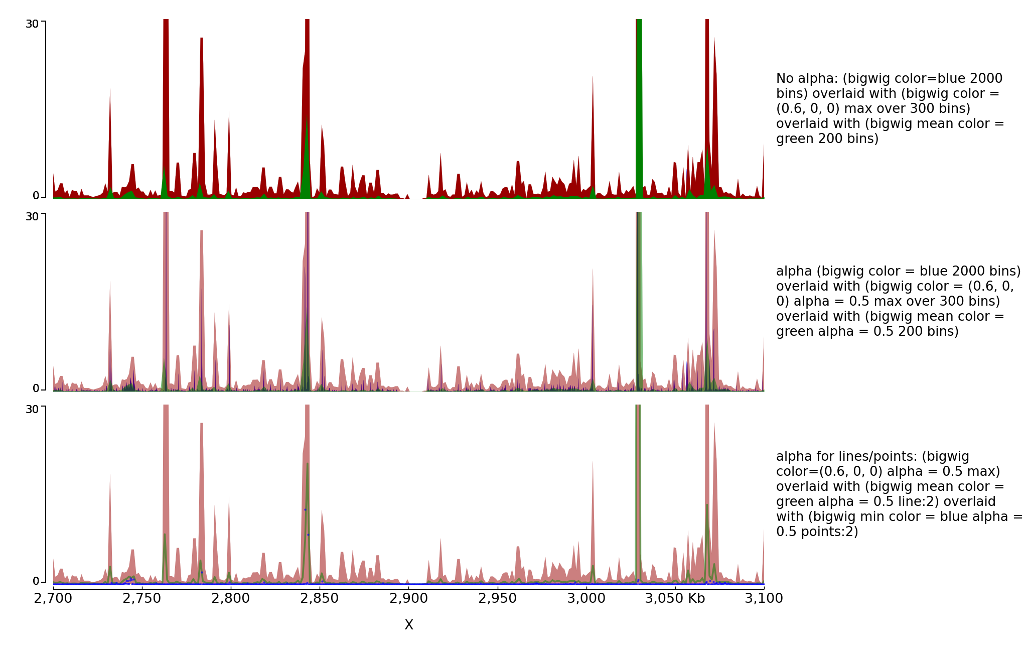
You can also overlay bigwig with or without transparency.
代码
文本
[ ]
[test bigwig]
file = bigwig2_X_2.5e6_3.5e6.bw
color = blue
height = 7
title = No alpha: (bigwig color=blue 2000 bins) overlaid with (bigwig color = (0.6, 0, 0) max over 300 bins) overlaid with (bigwig mean color = green 200 bins)
number_of_bins = 2000
min_value = 0
max_value = 30

[test bigwig max]
file = bigwig2_X_2.5e6_3.5e6.bw
color = (0.6, 0, 0)
summary_method = max
number_of_bins = 300
overlay_previous = share-y

[test bigwig mean]
file = bigwig2_X_2.5e6_3.5e6.bw
color = green
type = fill
number_of_bins = 200
overlay_previous = share-y

[spacer]

[test bigwig]
file = bigwig2_X_2.5e6_3.5e6.bw
color = blue
height = 7
title = alpha (bigwig color = blue 2000 bins) overlaid with (bigwig color = (0.6, 0, 0) alpha = 0.5 max over 300 bins) overlaid with (bigwig mean color = green alpha = 0.5 200 bins)
number_of_bins = 2000
min_value = 0
max_value = 30

[test bigwig max]
file = bigwig2_X_2.5e6_3.5e6.bw
color = (0.6, 0, 0)
alpha = 0.5
summary_method = max
number_of_bins = 300
overlay_previous = share-y

[test bigwig mean]
file = bigwig2_X_2.5e6_3.5e6.bw
color = green
alpha = 0.5
type = fill
number_of_bins = 200
overlay_previous = share-y

[spacer]

[test bigwig]
file = bigwig2_X_2.5e6_3.5e6.bw
height = 7
title = alpha for lines/points: (bigwig color=(0.6, 0, 0) alpha = 0.5 max) overlaid with (bigwig mean color = green alpha = 0.5 line:2) overlaid with (bigwig min color = blue alpha = 0.5 points:2)
color = (0.6, 0, 0)
alpha = 0.5
summary_method = max
number_of_bins = 300
min_value = 0
max_value = 30

[test bigwig mean]
file = bigwig2_X_2.5e6_3.5e6.bw
color = green
type = line:2
alpha = 0.5
summary_method = mean
number_of_bins = 300
overlay_previous = share-y

[test bigwig min]
file = bigwig2_X_2.5e6_3.5e6.bw
color = blue
summary_method = min
number_of_bins = 1000
type = points:3
alpha = 0.5
overlay_previous = share-y

[x-axis]
代码
文本
[ ]
! pyGenomeTracks --tracks alpha.ini --region X:2700000-3100000 --trackLabelFraction 0.2 --dpi 130 -o master_alpha.png
代码
文本

figure8

代码
文本

Examples with bed and gtf

Here is an example to explain the parameters for bed and gtf:
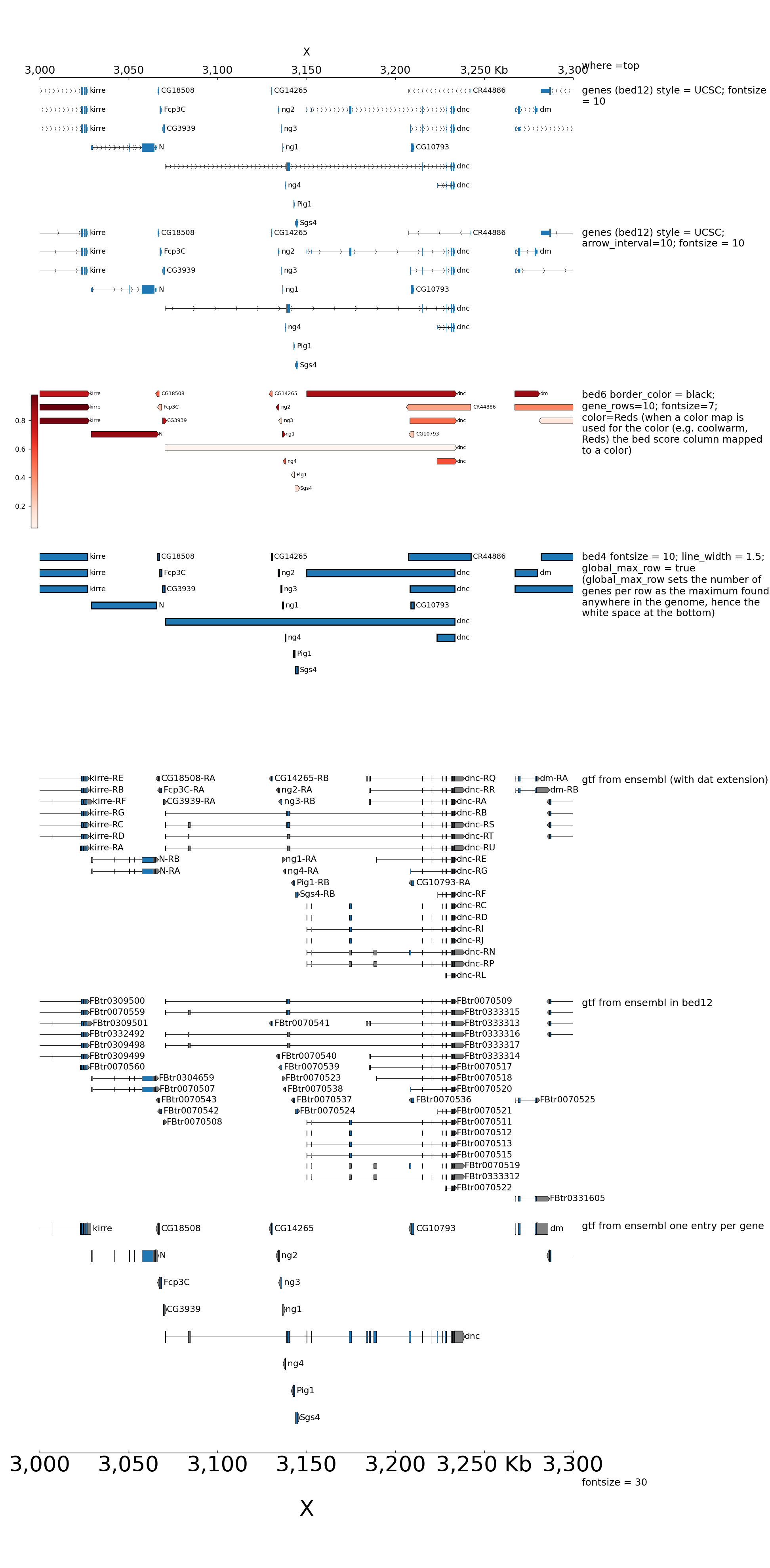
代码
文本
[ ]
[x-axis]
where = top
title = where =top

[spacer]
height = 0.05

[genes 2]
file = dm3_genes.bed.gz
height = 7
title = genes (bed12) style = UCSC; fontsize = 10
style = UCSC
fontsize = 10

[genes 2bis]
file = dm3_genes.bed.gz
height = 7
title = genes (bed12) style = UCSC; arrow_interval=10; fontsize = 10
style = UCSC
arrow_interval = 10
fontsize = 10

[spacer]
height = 1

[test bed6]
file = dm3_genes.bed6.gz
height = 7
title = bed6 border_color = black; gene_rows=10; fontsize=7; color=Reds (when a color map is used for the color (e.g. coolwarm, Reds) the bed score column mapped to a color)
fontsize = 7
file_type = bed
color = Reds
border_color = black
gene_rows = 10

[spacer]
height = 1

[test bed4]
file = dm3_genes.bed4.gz
height = 10
title = bed4 fontsize = 10; line_width = 1.5; global_max_row = true (global_max_row sets the number of genes per row as the maximum found anywhere in the genome, hence the white space at the bottom)
fontsize = 10
file_type = bed
global_max_row = true
line_width = 1.5

[spacer]
height = 1

[test gtf]
file = dm3_subset_BDGP5.78_gtf.dat
height = 10
title = gtf from ensembl (with dat extension)
fontsize = 12
file_type = gtf

[spacer]
height = 1

[test bed]
file = dm3_subset_BDGP5.78_asbed_sorted.bed.gz
height = 10
title = gtf from ensembl in bed12
fontsize = 12
file_type = bed

[spacer]
height = 1

[test gtf collapsed]
file = dm3_subset_BDGP5.78.gtf.gz
height = 10
title = gtf from ensembl one entry per gene
merge_transcripts = true
prefered_name = gene_name
fontsize = 12
file_type = gtf

[spacer]
height = 1

[x-axis]
fontsize = 30
title = fontsize = 30
代码
文本
[ ]
! pyGenomeTracks --tracks bed_and_gtf_tracks.ini --region X:3000000-3300000 --trackLabelFraction 0.2 --width 38 --dpi 130 -o master_bed_and_gtf.png
代码
文本

figure9

代码
文本

By default, when bed are displayed and interval are stranded, the arrowhead which indicates the direction is plotted outside of the interval. Here is an example to show how to put it inside:
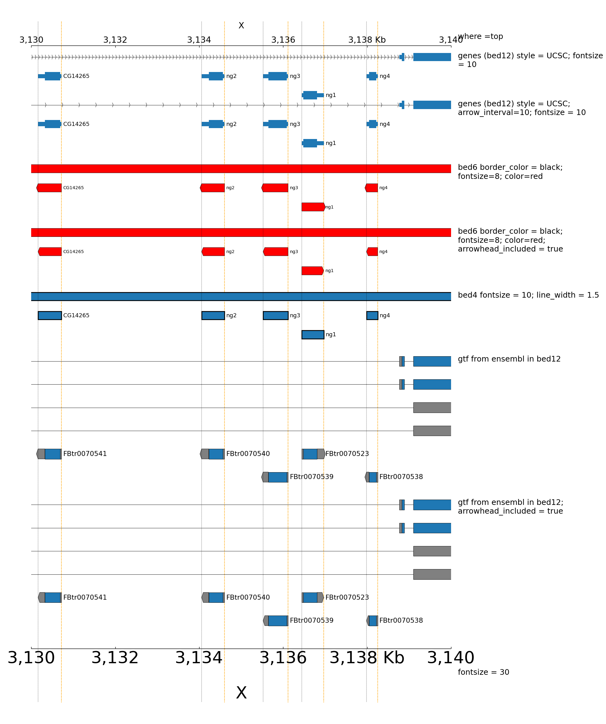
代码
文本
[ ]
[x-axis]
where = top
title = where =top

[spacer]
height = 0.05

[genes 2]
file = dm3_genes.bed.gz
height = 3
title = genes (bed12) style = UCSC; fontsize = 10
style = UCSC
fontsize = 10

[genes 2bis]
file = dm3_genes.bed.gz
height = 3
title = genes (bed12) style = UCSC; arrow_interval=10; fontsize = 10
style = UCSC
arrow_interval = 10
fontsize = 10

[spacer]
height = 1

[test bed6]
file = dm3_genes.bed6.gz
height = 3
title = bed6 border_color = black; fontsize=8; color=red
fontsize = 8
file_type = bed
color = red
border_color = black

[spacer]
height = 1

[test bed6 arrowhead_included]
file = dm3_genes.bed6.gz
height = 3
title = bed6 border_color = black; fontsize=8; color=red; arrowhead_included = true
fontsize = 8
file_type = bed
color = red
border_color = black
arrowhead_included = true

[spacer]
height = 1

[test bed4]
file = dm3_genes.bed4.gz
height = 3
title = bed4 fontsize = 10; line_width = 1.5
fontsize = 10
file_type = bed
line_width = 1.5

[spacer]
height = 1

[test bed]
file = dm3_subset_BDGP5.78_asbed_sorted.bed.gz
height = 8
title = gtf from ensembl in bed12
fontsize = 12
file_type = bed

[spacer]
height = 1

[test bed]
file = dm3_subset_BDGP5.78_asbed_sorted.bed.gz
height = 8
title = gtf from ensembl in bed12; arrowhead_included = true
fontsize = 12
file_type = bed
arrowhead_included = true

[spacer]
height = 1

[x-axis]
fontsize = 30
title = fontsize = 30

[vlines]
type = vlines
file = dm3_genes.bed4.gz
line_style = dotted

[second_vlines]
type = vlines
file = dm3_genes_end.bed
line_width = 1
color = orange
zorder = -100
代码
文本
[ ]
! pyGenomeTracks --tracks bed_arrow_tracks.ini --region X:3130000-3140000 --trackLabelFraction 0.2 --width 38 --dpi 130 -o master_bed_arrow_zoom.png
代码
文本

figure10

代码
文本

When genes are displayed with the default style (flybase), the color and the height of UTR can be set:
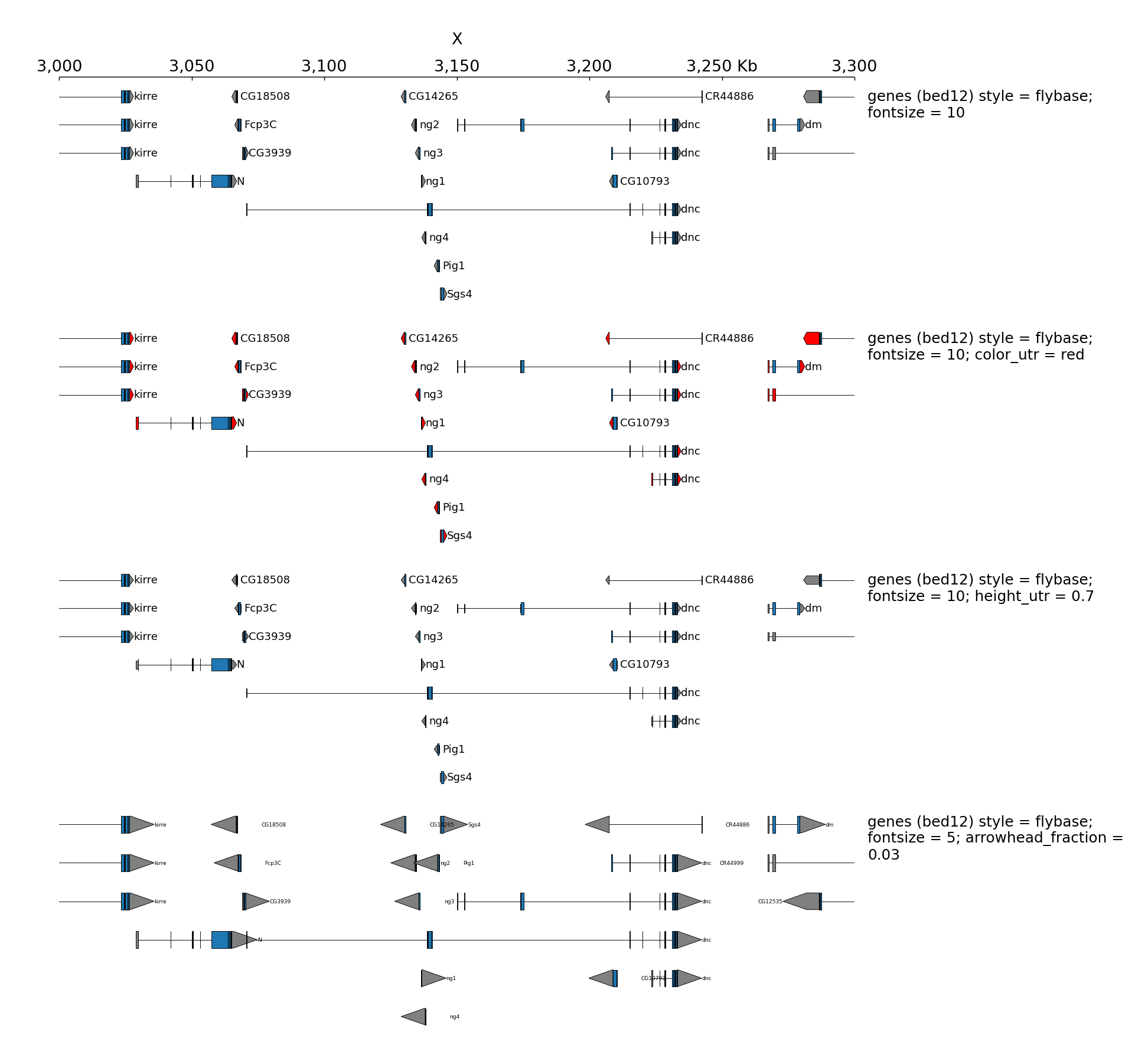
代码
文本
[ ]
[x-axis]
where = top

[spacer]
height = 0.05

[genes 0]
file = dm3_genes.bed.gz
height = 7
title = genes (bed12) style = flybase; fontsize = 10
style = flybase
fontsize = 10

[spacer]
height = 1

[genes 1]
file = dm3_genes.bed.gz
height = 7
title = genes (bed12) style = flybase; fontsize = 10; color_utr = red
style = flybase
fontsize = 10
color_utr = red

[spacer]
height = 1

[genes 2]
file = dm3_genes.bed.gz
height = 7
title = genes (bed12) style = flybase; fontsize = 10; height_utr = 0.7
style = flybase
fontsize = 10
height_utr = 0.7

[spacer]
height = 1

[genes 3]
file = dm3_genes.bed.gz
height = 7
title = genes (bed12) style = flybase; fontsize = 5; arrowhead_fraction = 0.03
style = flybase
fontsize = 5
arrowhead_fraction = 0.03
all_labels_inside = true
代码
文本
[ ]
! pyGenomeTracks --tracks bed_flybase_tracks.ini --region X:3000000-3300000 --trackLabelFraction 0.2 --width 38 --dpi 130 -o master_bed_flybase.png
代码
文本

figure11

代码
文本

Examples with 4C-seq

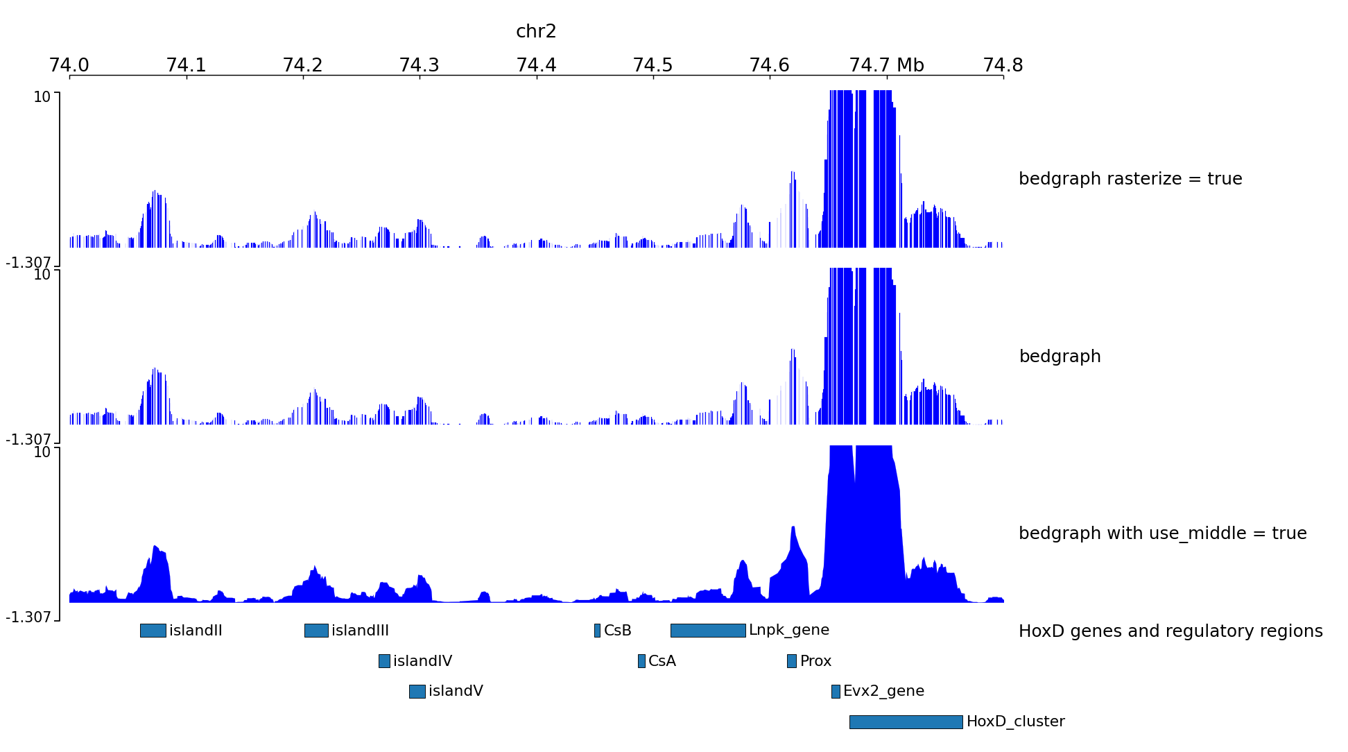
The output file of some 4C-seq pipeline are bedgraph where the coordinates are the coordinates of the fragment. In these cases, it can be interesting to remove the regions absent from the file and just link the middle of the fragments together instead of plotting a rectangle for each fragment. Here is an example of the option use_middle.

代码
文本
[ ]
[x-axis]
where = top

[spacer]
height = 0.05

[test bedgraph]
file = GSM3182416_E12DHL_WT_Hoxd11vp.bedgraph.gz
color = blue
height = 5
title = bedgraph rasterize = true
rasterize = true
max_value = 10

[test bedgraph]
file = GSM3182416_E12DHL_WT_Hoxd11vp.bedgraph.gz
color = blue
height = 5
title = bedgraph
max_value = 10

[test bedgraph use middle]
file = GSM3182416_E12DHL_WT_Hoxd11vp.bedgraph.gz
color = blue
height = 5
title = bedgraph with use_middle = true
max_value = 10
use_middle = true

[genes]
file = HoxD_cluster_regulatory_regions_mm10.bed
height = 3
title = HoxD genes and regulatory regions
代码
文本

We can generate two zooms using a bed instead of regions:
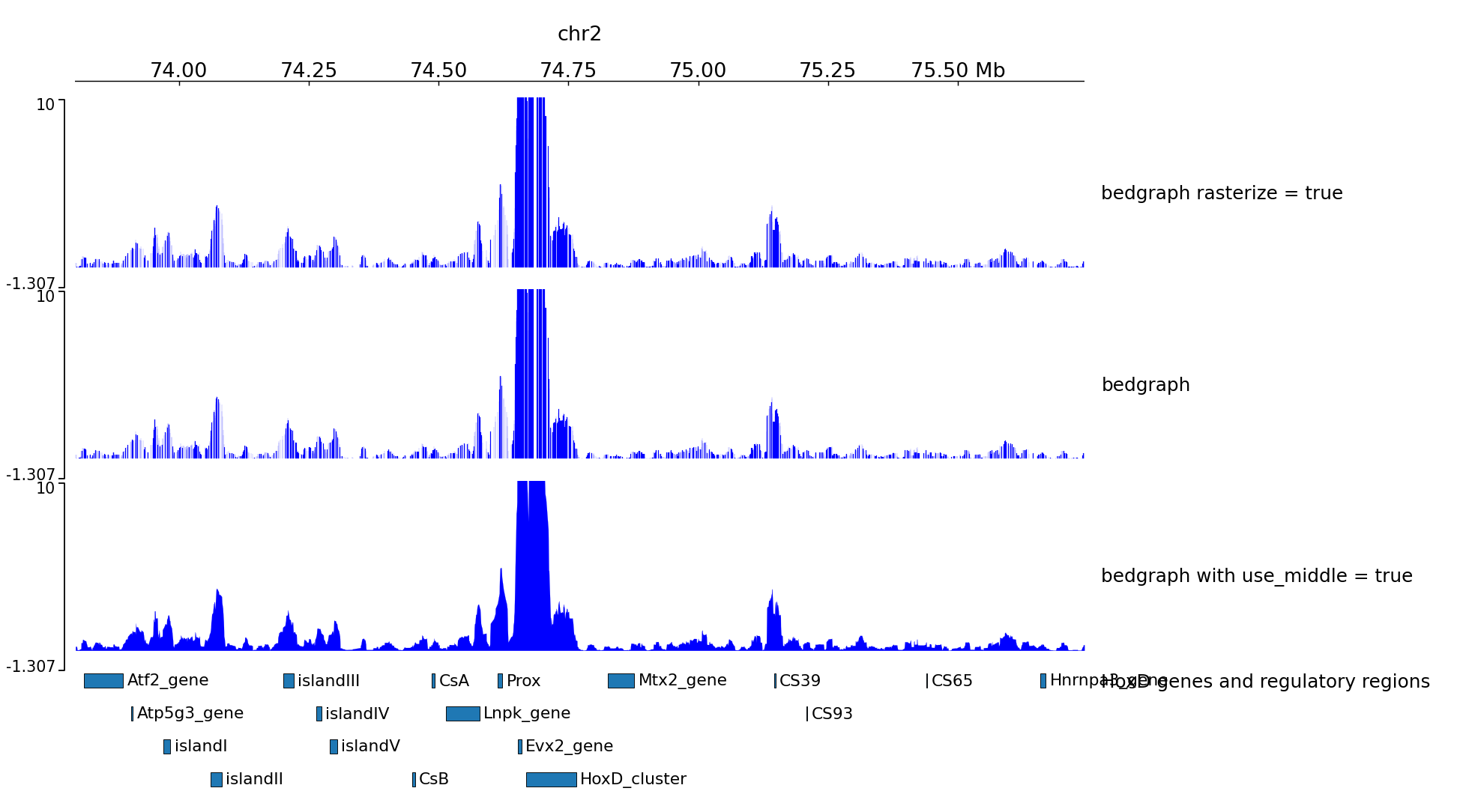
代码
文本
[ ]
track type=bed name=regions_to_plot
chr2 73800000 75744000
chr2 74000000 74800000
代码
文本
[ ]
! pyGenomeTracks --tracks bedgraph_useMid.ini --BED regions_imbricated_chr2.bed --trackLabelFraction 0.2 --width 38 --dpi 130 -o master_bedgraph_useMid.png
代码
文本

figure12 figure13

代码
文本

Examples with peaks

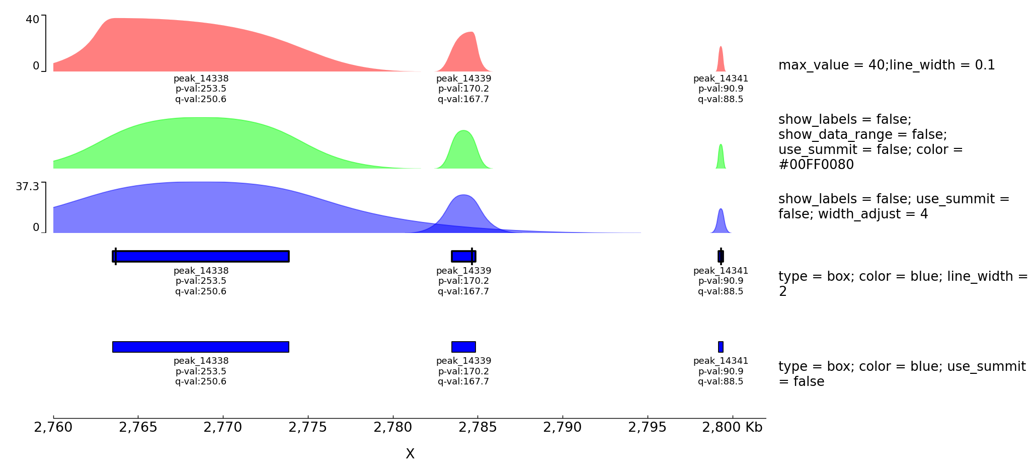
pyGenomeTracks has an option to plot peaks using MACS2 narrowPeak format.

The following is an example of the output in which the peak shape is drawn based on the start, end, summit and height of the peak.
代码
文本
[ ]
[narrow]
file = test2.narrowPeak
height = 4
max_value = 40
line_width = 0.1
title = max_value = 40;line_width = 0.1

[narrow 2]
file = test2.narrowPeak
height = 2
show_labels = false
show_data_range = false
color = #00FF0080
use_summit = false
title = show_labels = false; show_data_range = false; use_summit = false; color = #00FF0080

[spacer]

[narrow 3]
file = test2.narrowPeak
height = 2
show_labels = false
color = #0000FF80
use_summit = false
width_adjust = 4
title = show_labels = false; use_summit = false; width_adjust = 4

[spacer]

[narrow 4]
file = test2.narrowPeak
height = 3
type = box
color = blue
line_width = 2
title = type = box; color = blue; line_width = 2

[spacer]

[narrow 5]
file = test2.narrowPeak
height = 3
type = box
color = blue
use_summit = false
title = type = box; color = blue; use_summit = false

[x-axis]
代码
文本
[ ]
! pyGenomeTracks --tracks narrow_peak2.ini --region X:2760000-2802000 --trackLabelFraction 0.2 --dpi 130 -o master_narrowPeak2.png
代码
文本

figure13

代码
文本

Example with horizontal lines

代码
文本
[ ]
[test hlines]
color = red
line_width = 2
line_style = dashed
y_values = 10, 200
min_value = 0
show_data_range = true
height = 5
title = hlines: color = red; line_width = 2; line_style = dashed; y_values = 10, 200
file_type = hlines

[spacer]

[test bigwig fill]
file = bigwig2_X_2.5e6_3.5e6.bw
color = gray
height = 2
type = fill
title = bigwig: gray fill overlayed with hlines at 10 and 200 blue dotted
max_value = 50

[test hlines ovelayed]
color = blue
line_style = dotted
y_values = 10, 200
overlay_previous = share-y
file_type = hlines

[spacer]

[x-axis]
代码
文本
[ ]
! pyGenomeTracks --tracks hlines.ini --region X:2700000-3100000 --trackLabelFraction 0.2 --dpi 130 -o master_hlines.png
代码
文本

figure15

代码
文本

Examples with Epilogos

pyGenomeTracks can be used to visualize epigenetic states (for example from chromHMM) as epilogos. For more information see: https://epilogos.altiusinstitute.org/

To plot epilogos a qcat file is needed. This file can be crated using the epilogos software (https://github.com/Altius/epilogos).

An example track file for epilogos looks like:

代码
文本
[ ]
[epilogos]
file = epilog.qcat.bgz
height = 5
title = height=5; categories_file=epilog_cats.json

[x-axis]
代码
文本
[ ]
! pyGenomeTracks --tracks epilogos_track.ini --region X:3100000-3150000 -o epilogos_track.png
代码
文本

figure16

代码
文本

The color of the bars can be set by using a json file. The structure of the file is like this:

代码
文本
[ ]
{
"categories":{
"1":["Active TSS","#ff0000"],
"2":["Flanking Active TSS","#ff4500"],
"3":["Transcr at gene 5\" and 3\"","#32cd32"],
"4":["Strong transcription","#008000"],
"5":["Weak transcription","#006400"],
"6":["Genic enhancers","#c2e105"],
"7":["Enhancers","#ffff00"],
"8":["ZNF genes & repeats","#66cdaa"],
"9":["Heterochromatin","#8a91d0"],
"10":["Bivalent/Poised TSS","#cd5c5c"],
"11":["Flanking Bivalent TSS/Enh","#e9967a"],
"12":["Bivalent Enhancer","#bdb76b"],
"13":["Repressed PolyComb","#808080"],
"14":["Weak Repressed PolyComb","#c0c0c0"],
"15":["Quiescent/Low","#ffffff"]
}
}
代码
文本

In the following examples the top epilogo has the custom colors and the one below is shown inverted.

代码
文本
[ ]
[epilogos]
file = epilog.qcat.bgz
height = 5
title = epilogos with custom colors
categories_file = epilog_cats.json

[epilogos inverted]
file = epilog.qcat.bgz
height = 5
title = epilogos inverted
orientation = inverted

[x-axis]
代码
文本
[ ]
! pyGenomeTracks --tracks epilogos_track2.ini --region X:3100000-3150000 -o epilogos_track2.png
代码
文本

figure16

代码
文本

Examples with multiple options

A comprehensive example of pyGenomeTracks can be found as part of our automatic testing. Note, that pyGenomeTracks also allows the combination of multiple tracks into one using the parameter: overlay_previous = yes or overlay_previous = share-y. In the second option the y-axis of the tracks that overlays is the same as the track being overlay. Multiple tracks can be overlay together.
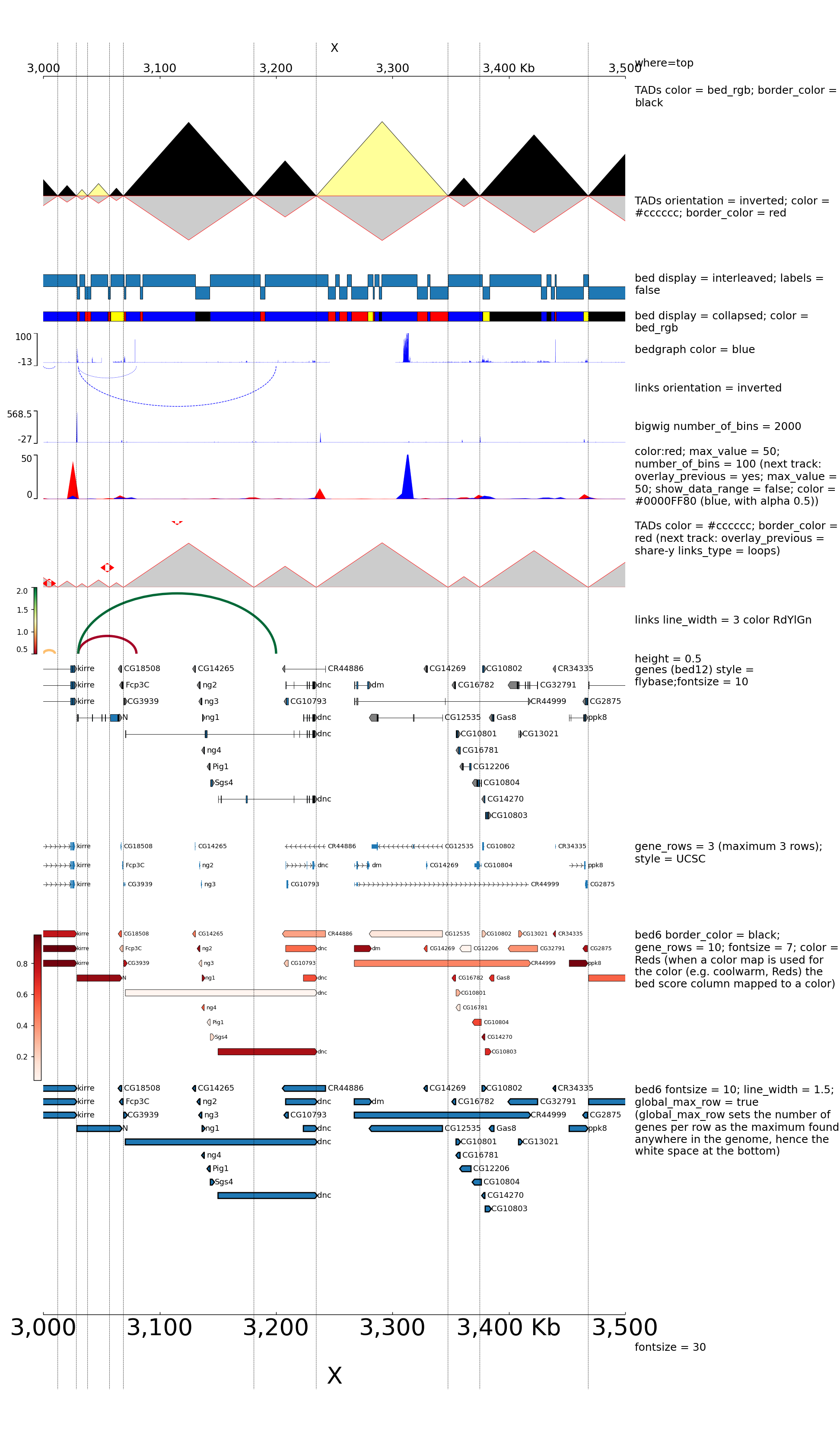
figure2

The configuration file for this image is:

代码
文本
[ ]
[x-axis]
where = top
title = where=top

[spacer]
height = 0.05

[tads]
file = tad_classification.bed
title = TADs color = bed_rgb; border_color = black
file_type = domains
border_color = black
color = bed_rgb
height = 5

[tads 2]
file = tad_classification.bed
title = TADs orientation = inverted; color = #cccccc; border_color = red
file_type = domains
border_color = red
color = #cccccc
orientation = inverted
height = 3

[spacer]
height = 0.5

[tad state]
file = chromatinStates_kc.bed.gz
height = 1.2
title = bed display = interleaved; labels = false
display = interleaved
labels = false

[spacer]
height = 0.5

[tad state]
file = chromatinStates_kc.bed.gz
height = 0.5
title = bed display = collapsed; color = bed_rgb
labels = false
color = bed_rgb
display = collapsed

[spacer]
height = 0.5

[test bedgraph]
file = bedgraph_chrx_2e6_5e6.bg
color = blue
height = 1.5
title = bedgraph color = blue
max_value = 100

[test arcs]
file = test.arcs
title = links orientation = inverted
orientation = inverted
line_style = dashed
height = 2

[test bigwig]
file = bigwig2_X_2.5e6_3.5e6.bw
color = blue
height = 1.5
title = bigwig number_of_bins = 2000
number_of_bins = 2000

[spacer]

[test bigwig overlay]
file = bigwig2_X_2.5e6_3.5e6.bw
color = red
title = color:red; max_value = 50; number_of_bins = 100 (next track: overlay_previous = yes; max_value = 50; show_data_range = false; color = #0000FF80 (blue, with alpha 0.5))
min_value = 0
max_value = 50
height = 2
number_of_bins = 100

[test bigwig overlay]
file = bigwig_chrx_2e6_5e6.bw
color = #0000FF80
title =
min_value = 0
max_value = 50
show_data_range = false
overlay_previous = yes
number_of_bins = 100

[spacer]
height = 1

[tads 3]
file = tad_classification.bed
title = TADs color = #cccccc; border_color = red (next track: overlay_previous = share-y links_type = loops)
file_type = domains
border_color = red
color = #cccccc
height = 3

[test arcs overlay]
file = test.arcs
color = red
line_width = 10
links_type = loops
overlay_previous = share-y

[test arcs]
file = test.arcs
line_width = 3
color = RdYlGn
title = links line_width = 3 color RdYlGn
height = 3

[spacer]
height = 0.5
title = height = 0.5

[genes 2]
file = dm3_genes.bed.gz
height = 7
title = genes (bed12) style = flybase;fontsize = 10
style = flybase
fontsize = 10

[spacer]
height = 1

[test gene rows]
file = dm3_genes.bed.gz
height = 3
title = gene_rows = 3 (maximum 3 rows); style = UCSC
fontsize = 8
style = UCSC
gene_rows = 3

[spacer]
height = 1

[test bed6]
file = dm3_genes.bed6.gz
height = 7
title = bed6 border_color = black; gene_rows = 10; fontsize = 7; color = Reds (when a color map is used for the color (e.g. coolwarm, Reds) the bed score column mapped to a color)
fontsize = 7
file_type = bed
color = Reds
border_color = black
gene_rows = 10

[test bed6]
file = dm3_genes.bed6.gz
height = 10
title = bed6 fontsize = 10; line_width = 1.5; global_max_row = true (global_max_row sets the number of genes per row as the maximum found anywhere in the genome, hence the white space at the bottom)
fontsize = 10
file_type = bed
global_max_row = true
line_width = 1.5

[x-axis]
fontsize = 30
title = fontsize = 30

[vlines]
file = tad_classification.bed
type = vlines
代码
文本
[ ]
! pyGenomeTracks --tracks browser_tracks.ini --region X:3000000-3500000 --trackLabelFraction 0.2 --width 38 --dpi 130 -o master_plot.png
代码
文本

Examples with multiple options for bigwig tracks
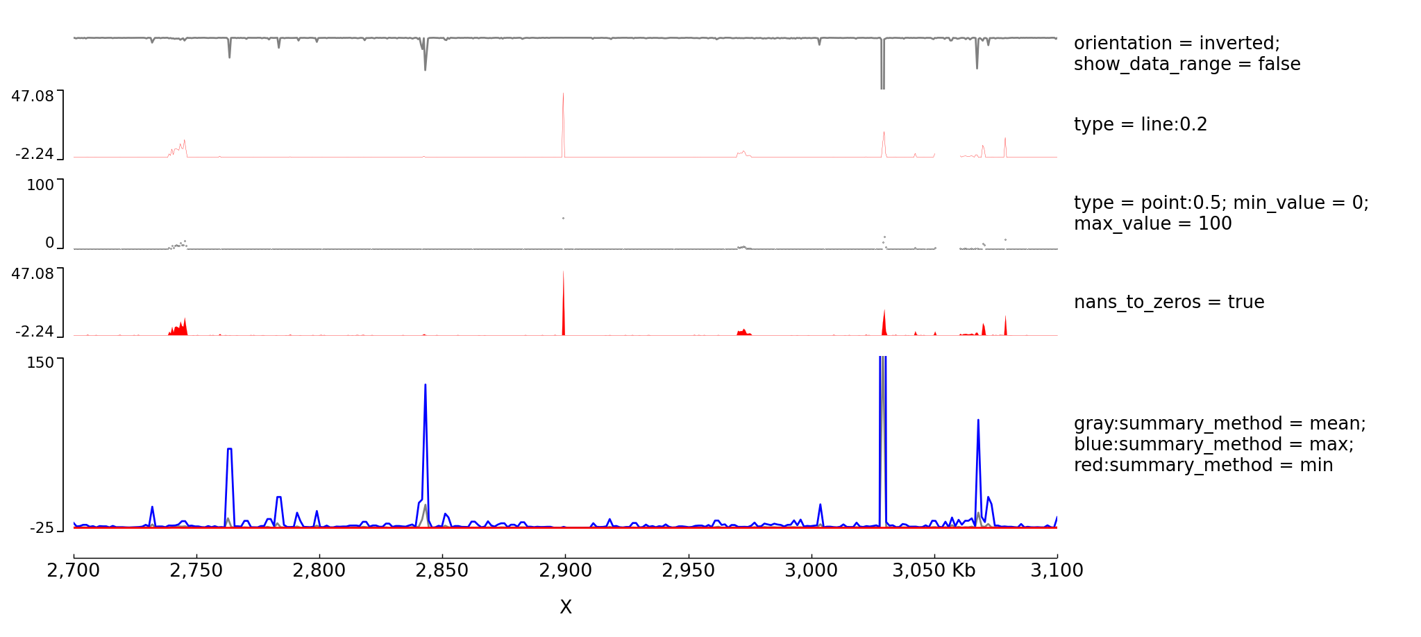
figure1 The configuration file for this image is:

代码
文本
[ ]
[test bigwig lines]
file = bigwig2_X_2.5e6_3.5e6.bw
color = gray
height = 2
type = line
title = orientation = inverted; show_data_range = false
orientation = inverted
show_data_range = false
max_value = 50

[test bigwig lines:0.2]
file = bigwig_chrx_2e6_5e6.bw
color = red
height = 2
type = line:0.2
title = type = line:0.2
min_value = auto
max_value = auto

[spacer]

[test bigwig points]
file = bigwig_chrx_2e6_5e6.bw
color = black
height = 2
min_value = 0
max_value = 100
type = points:0.5
title = type = point:0.5; min_value = 0; max_value = 100

[spacer]

[test bigwig nans to zeros]
file = bigwig_chrx_2e6_5e6.bw
color = red
height = 2
nans_to_zeros = true
title = nans_to_zeros = true

[spacer]

[test bigwig mean]
file = bigwig2_X_2.5e6_3.5e6.bw
color = gray
height = 5
title = gray:summary_method = mean; blue:summary_method = max; red:summary_method = min
type = line
summary_method = mean
max_value = 150
min_value = -5
show_data_range = false
number_of_bins = 300

[test bigwig max]
file = bigwig2_X_2.5e6_3.5e6.bw
#title = test
color = blue
type = line
summary_method = max
max_value = 150
min_value = -15
show_data_range = false
overlay_previous = share-y
number_of_bins = 300

[test bigwig min]
file = bigwig2_X_2.5e6_3.5e6.bw
color = red
type = line
summary_method = min
max_value = 150
min_value = -25
overlay_previous = share-y
number_of_bins = 300

[spacer]

[x-axis]
代码
文本
[ ]
! pyGenomeTracks --tracks bigwig.ini --region X:2700000-3100000 --trackLabelFraction 0.2 --dpi 130 -o master_bigwig.png
代码
文本

Examples with Hi-C data

The following is an example with Hi-C data overlay with topologically associating domains (TADs) and a bigwig file.

代码
文本
[ ]
[x-axis]
where = top

[hic matrix]
file = hic_data.h5
title = Hi-C data
# depth is the maximum distance plotted in bp. In Hi-C tracks
# the height of the track is calculated based on the depth such
# that the matrix does not look deformed
depth = 300000
transform = log1p
file_type = hic_matrix

[tads]
file = domains.bed
display = triangles
border_color = black
color = none
# the tads are overlay over the hic-matrix
# the share-y options sets the y-axis to be shared
# between the Hi-C matrix and the TADs.
overlay_previous = share-y

[spacer]

[bigwig file test]
file = bigwig.bw
# height of the track in cm (optional value)
height = 4
title = ChIP-seq
min_value = 0
max_value = 30
代码
文本
[ ]
! pyGenomeTracks --tracks hic_track.ini -o hic_track.png --region chrX:2500000-3500000
代码
文本

Here is an example where the height was set or not set and the heatmap was rasterized (default) or not rasterized (the dpi was set very low just to show the impact of the parameter).

代码
文本
[ ]
[hic matrix]
file = Li_et_al_2015.cool
title = depth = 200000; transform = log1p; min_value = 5; height = 5
depth = 200000
min_value = 5
transform = log1p
file_type = hic_matrix
show_masked_bins = false
height = 5

[hic matrix 2]
file = Li_et_al_2015.h5
title = same but orientation=inverted; no height
depth = 200000
min_value = 5
transform = log1p
file_type = hic_matrix
show_masked_bins = false
orientation = inverted

[spacer]
height = 0.5

[hic matrix 3]
file = Li_et_al_2015.h5
title = same rasterize = false
depth = 200000
min_value = 5
transform = log1p
file_type = hic_matrix
rasterize = false
show_masked_bins = false

[x-axis]
代码
文本
[ ]
! pyGenomeTracks --tracks browser_tracks_hic_rasterize_height.ini --region X:2500000-2600000 --trackLabelFraction 0.23 --width 38 --dpi 10 -o master_plot_hic_rasterize_height.pdf
代码
文本

The output is available here: master_plot_hic_rasterize_height.pdf.

This examples is where the overlay tracks are more useful. Notice that any track can be overlay over a Hi-C matrix. Most useful is to overlay TADs or to overlay links using the triangles option that will point in the Hi-C matrix the pixel with the link contact. When overlaying links and TADs is useful to set overlay_previous=share-y such that the two tracks match the positions. This is not required when overlying other type of data like a bigwig file that has a different y-scale.
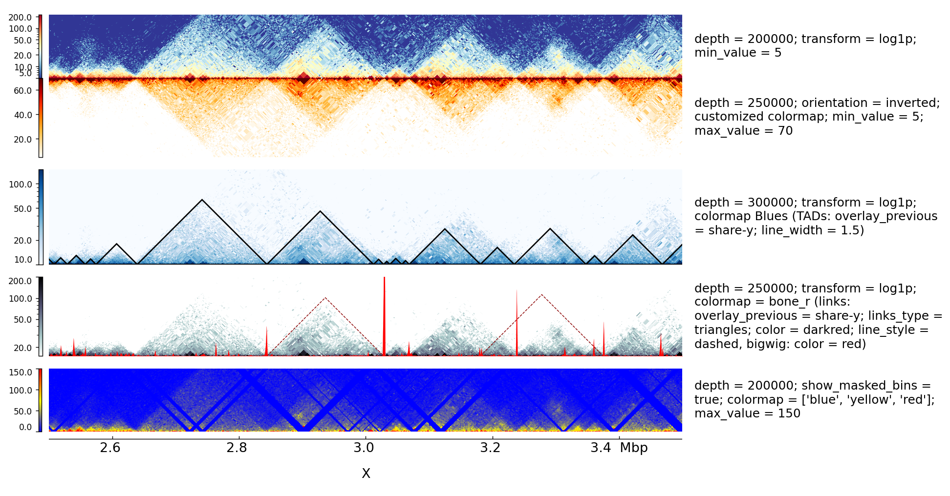
figure3

The configuration file for this image is:

代码
文本
[ ]
[hic matrix]
file = Li_et_al_2015.h5
title = depth = 200000; transform = log1p; min_value = 5
depth = 200000
min_value = 5
transform = log1p
file_type = hic_matrix
show_masked_bins = false

[hic matrix]
file = Li_et_al_2015.h5
title = depth = 250000; orientation = inverted; customized colormap; min_value = 5; max_value = 70
min_value = 5
max_value = 70
depth = 250000
colormap = ['white', (1, 0.88, .66), (1, 0.74, 0.25), (1, 0.5, 0), (1, 0.19, 0), (0.74, 0, 0), (0.35, 0, 0)]
file_type = hic_matrix
show_masked_bins = false
orientation = inverted

[spacer]
height = 0.5

[hic matrix]
file = Li_et_al_2015.h5
title = depth = 300000; transform = log1p; colormap Blues (TADs: overlay_previous = share-y; line_width = 1.5)
colormap = Blues
min_value = 10
max_value = 150
depth = 300000
transform = log1p
file_type = hic_matrix

[tads]
file = tad_classification.bed
#title = TADs color = none; border_color = black
file_type = domains
border_color = black
color = none
height = 5
line_width = 1.5
overlay_previous = share-y
show_data_range = false

[spacer]
height = 0.5

[hic matrix]
file = Li_et_al_2015.h5
title = depth = 250000; transform = log1p; colormap = bone_r (links: overlay_previous = share-y; links_type = triangles; color = darkred; line_style = dashed, bigwig: color = red)
colormap = bone_r
min_value = 15
max_value = 200
depth = 250000
transform = log1p
file_type = hic_matrix
show_masked_bins = false

[test arcs]
file = links2.links
title =
links_type = triangles
line_style = dashed
overlay_previous = share-y
line_width = 0.8
color = darkred
show_data_range = false


[test bigwig]
file = bigwig2_X_2.5e6_3.5e6.bw
color = red
height = 4
title =
overlay_previous = yes
min_value = 0
max_value = 50
show_data_range = false

[spacer]
height = 0.5

[hic matrix]
file = Li_et_al_2015.h5
title = depth = 200000; show_masked_bins = true; colormap = ['blue', 'yellow', 'red']; max_value = 150
depth = 200000
colormap = ['blue', 'yellow', 'red']
max_value = 150
file_type = hic_matrix
show_masked_bins = true

[spacer]
height = 0.1

[x-axis]
代码
文本
[ ]
! pyGenomeTracks --tracks browser_tracks_hic.ini --region X:2500000-3500000 --trackLabelFraction 0.23 --width 38 --dpi 130 -o master_plot_hic.png
代码
文本

figure18

代码
文本

Log transform and Operation Examples

With the parameter operation you can make operations between one or two files (here two bigwig files but this is also working with two bedgraph files). For example, difference, log ratio, scaling…
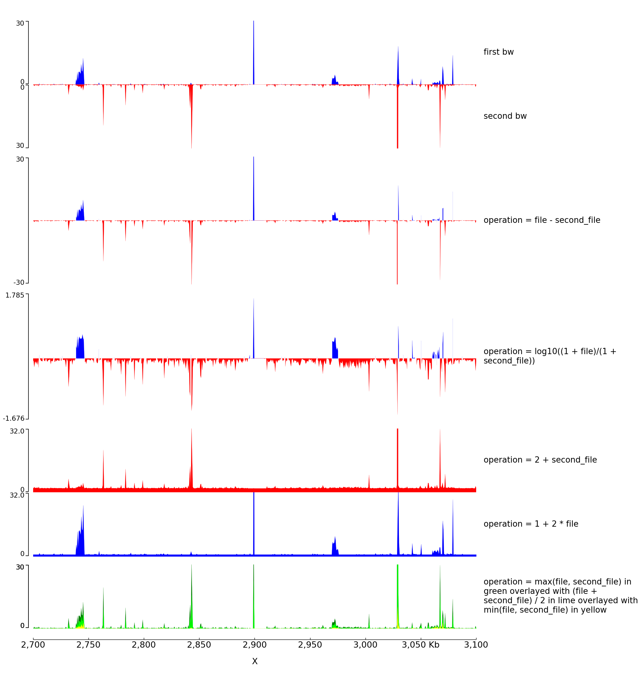
figure4

The configuration file for this image is:

代码
文本
[ ]
[test bigwig1]
file = bigwig_chrx_2e6_5e6.bw
second_file = bigwig2_X_2.5e6_3.5e6.bw
color = blue
height = 4
title = first bw
min_value = 0
max_value = 30

[test bigwig2]
file = bigwig2_X_2.5e6_3.5e6.bw
color = red
height = 4
title = second bw
min_value = 0
max_value = 30
orientation = inverted

[spacer]
height = 0.5

[test bigwig dif]
file = bigwig_chrx_2e6_5e6.bw
second_file = bigwig2_X_2.5e6_3.5e6.bw
color = blue
negative_color = red
height = 8
title = operation = file - second_file
operation = file - second_file
min_value = -30
max_value = 30
nans_to_zeros = true

[spacer]
height = 0.5

[test bigwig op]
file = bigwig_chrx_2e6_5e6.bw
second_file = bigwig2_X_2.5e6_3.5e6.bw
color = blue
negative_color = red
height = 8
title = operation = log10((1 + file)/(1 + second_file))
operation = log10((1 + file)/(1 + second_file))
nans_to_zeros = true

[spacer]
height = 0.5

[test bigwig op2]
file = bigwig_chrx_2e6_5e6.bw
second_file = bigwig2_X_2.5e6_3.5e6.bw
color = red
height = 4
title = operation = 2 + second_file
operation = 2 + second_file
nans_to_zeros = true
max_value = 32
min_value = 0

[test bigwig op2bis]
file = bigwig_chrx_2e6_5e6.bw
second_file = bigwig2_X_2.5e6_3.5e6.bw
color = blue
height = 4
title = operation = 1 + 2 * file
operation = 1 + 2 * file
nans_to_zeros = true
max_value = 32
min_value = 0

[spacer]
height = 0.5

[test bigwig op3]
file = bigwig_chrx_2e6_5e6.bw
second_file = bigwig2_X_2.5e6_3.5e6.bw
color = green
height = 4
title = operation = max(file, second_file) in green overlayed with (file + second_file) / 2 in lime overlayed with min(file, second_file) in yellow
operation = max(file, second_file)
nans_to_zeros = true
max_value = 30
min_value = 0

[test bigwig op4]
file = bigwig_chrx_2e6_5e6.bw
second_file = bigwig2_X_2.5e6_3.5e6.bw
color = lime
operation = (file + second_file) / 2
nans_to_zeros = true
overlay_previous = share-y

[test bigwig op5]
file = bigwig_chrx_2e6_5e6.bw
second_file = bigwig2_X_2.5e6_3.5e6.bw
color = yellow
operation = min(file, second_file)
nans_to_zeros = true
overlay_previous = share-y

[spacer]
height = 0.5


[x-axis]
代码
文本
[ ]
! pyGenomeTracks --tracks operation.ini --region X:2700000-3100000 --trackLabelFraction 0.2 --dpi 130 -o master_operation.png
代码
文本

With the parameter transformation you can log transform your data and decide to put on the y axis either the transformed values or the original values:
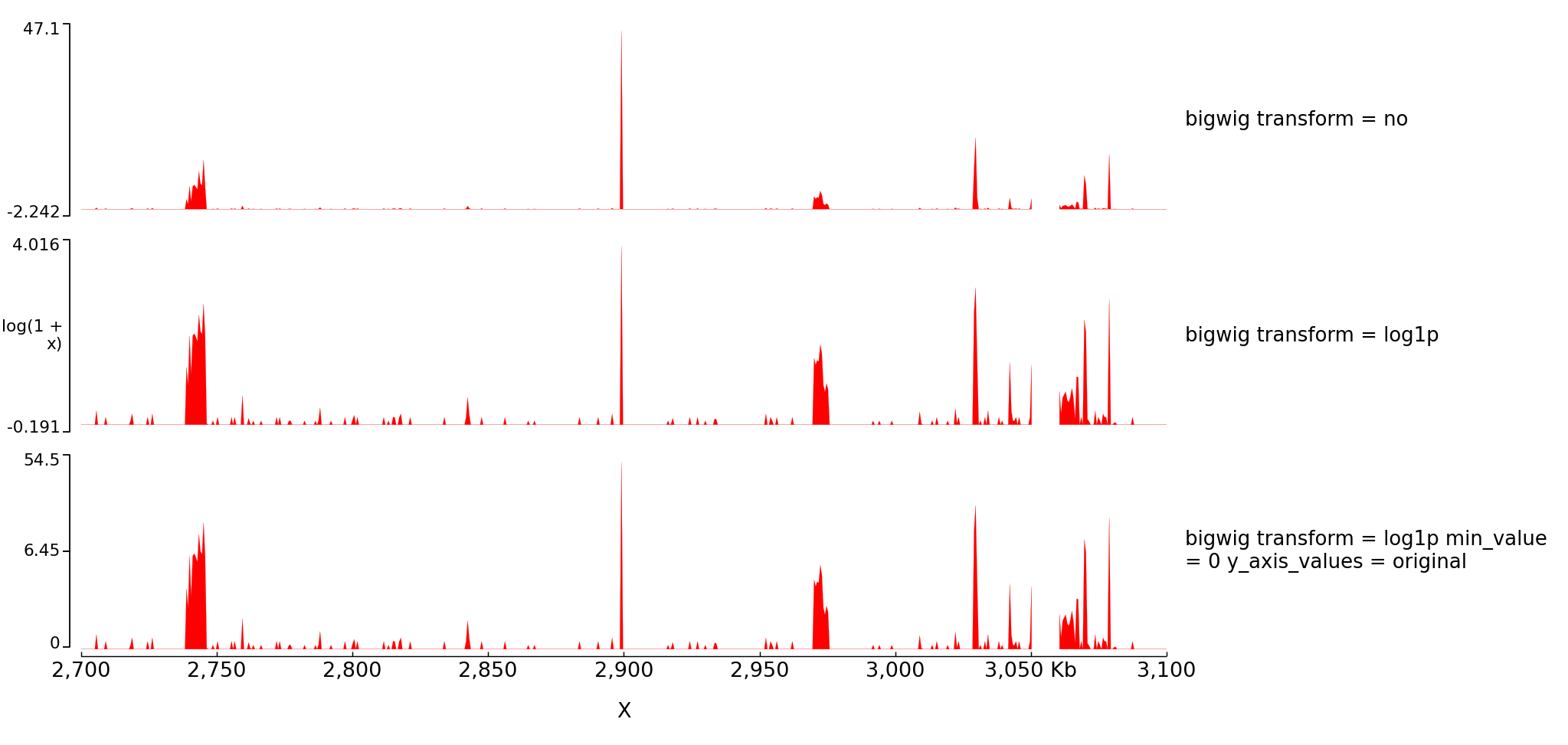
figure5

代码
文本

The configuration file for this image is:

代码
文本
[ ]
[test bigwig]
file = bigwig_chrx_2e6_5e6.bw
color = red
height = 5
transform = no
title = bigwig transform = no

[spacer]

[test bigwig log]
file = bigwig_chrx_2e6_5e6.bw
color = red
height = 5
transform = log1p
title = bigwig transform = log1p

[spacer]

[test bigwig log]
file = bigwig_chrx_2e6_5e6.bw
color = red
min_value = 0
height = 5
transform = log1p
title = bigwig transform = log1p min_value = 0 y_axis_values = original
y_axis_values = original

[x-axis]
代码
文本
[ ]
! pyGenomeTracks --tracks log1p.ini --region X:2700000-3100000 --trackLabelFraction 0.2 --dpi 130 -o master_log1p.png
代码
文本

With operation you can also do log transformation however nothing will be written on the left of the y axis:
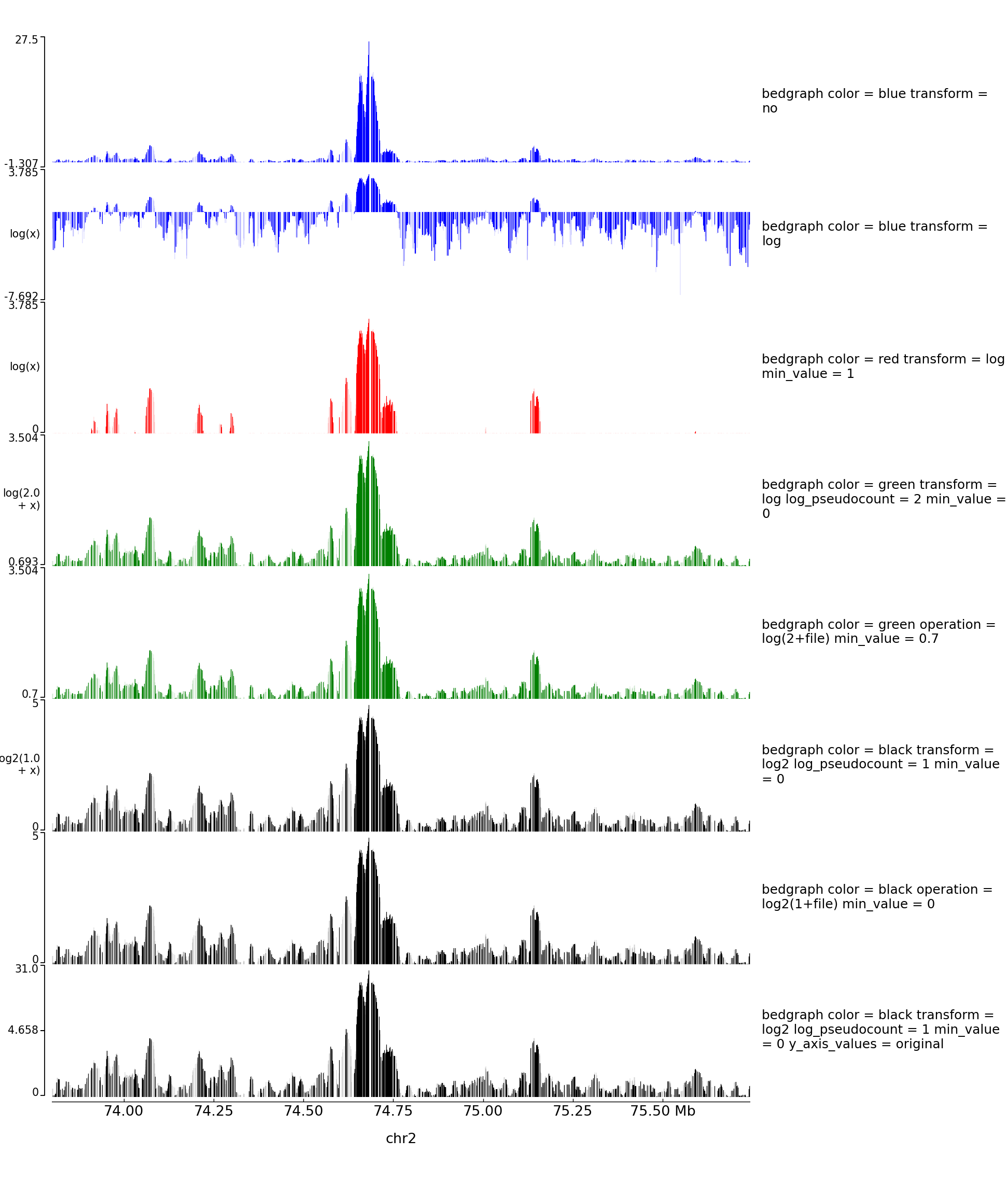
figure6

The configuration file for this image is:

代码
文本
[ ]
[test bedgraph]
file = GSM3182416_E12DHL_WT_Hoxd11vp.bedgraph.gz
color = blue
height = 5
title = bedgraph color = blue transform = no
transform = no

[test bedgraph]
file = GSM3182416_E12DHL_WT_Hoxd11vp.bedgraph.gz
color = blue
height = 5
title = bedgraph color = blue transform = log
transform = log

[test bedgraph]
file = GSM3182416_E12DHL_WT_Hoxd11vp.bedgraph.gz
color = red
height = 5
title = bedgraph color = red transform = log min_value = 1
min_value = 1
transform = log

[test bedgraph]
file = GSM3182416_E12DHL_WT_Hoxd11vp.bedgraph.gz
color = green
height = 5
title = bedgraph color = green transform = log log_pseudocount = 2 min_value = 0
transform = log
log_pseudocount = 2
min_value = 0

[test bedgraph with operation]
file = GSM3182416_E12DHL_WT_Hoxd11vp.bedgraph.gz
color = green
height = 5
title = bedgraph color = green operation = log(2+file) min_value = 0.7
operation = log(2+file)
min_value = 0.7

[test bedgraph]
file = GSM3182416_E12DHL_WT_Hoxd11vp.bedgraph.gz
color = black
height = 5
title = bedgraph color = black transform = log2 log_pseudocount = 1 min_value = 0
transform = log2
log_pseudocount = 1
min_value = 0

[test bedgraph]
file = GSM3182416_E12DHL_WT_Hoxd11vp.bedgraph.gz
color = black
height = 5
title = bedgraph color = black operation = log2(1+file) min_value = 0
operation = log2(1+file)
min_value = 0

[test bedgraph]
file = GSM3182416_E12DHL_WT_Hoxd11vp.bedgraph.gz
color = black
height = 5
title = bedgraph color = black transform = log2 log_pseudocount = 1 min_value = 0 y_axis_values = original
transform = log2
log_pseudocount = 1
min_value = 0
y_axis_values = original

[x-axis]
代码
文本
[ ]
! pyGenomeTracks --tracks log.ini --region chr2:73,800,000-75,744,000 --trackLabelFraction 0.2 --width 38 --dpi 130 -o master_log.png
代码
文本

References

  • Lopez-Delisle L, Rabbani L, Wolff J, Bhardwaj V, Backofen R, Grüning B, Ramírez F, Manke T. pyGenomeTracks: reproducible plots for multivariate genomic data sets. Bioinformatics. 2020 Aug 3:btaa692. doi: 10.1093/bioinformatics/btaa692. Epub ahead of print. PMID: 32745185.
代码
文本
中文
生物信息学
基因组
可视化
中文生物信息学基因组可视化
已赞2
本文被以下合集收录
生物信息学 Notebooks Collection
liyongge
更新于 2024-09-13
33 篇75 人关注
生信作图工具
liyongge
更新于 2024-04-01
6 篇1 人关注
推荐阅读
公开
GOplot:把你的差异表达基因富集分析结果画出来!
中文生物信息学
中文生物信息学
Judy Lin
发布于 2023-08-05
3 赞2 转存文件
公开
transPlotR:优雅地绘制基因转录本结构
生物信息学中文基因组转录组
生物信息学中文基因组转录组
Judy Lin
发布于 2023-08-05
1 赞1 转存文件2 评论