Diffusion probabilistic models - Applications to waveforms

Author : Philippe Esling (esling@ircam.fr)

This third notebook continues the exploration of diffusion probabilistic models [ 1 ] in our four notebook series.

1. Score matching and Langevin dynamics.
2. Diffusion probabilistic models and denoising
3. Applications to waveforms with WaveGrad
4. Implicit models to accelerate inference

Here, we quickly recall the basics of score matching [ 3 ] , Langevin dynamics and diffusion probabilistic models [ 1 ] seen in the previous notebooks, in order to discuss applications to waveform data, through the WaveGrad model [ 5 ]

Theoretical bases - quick recap

In this section we provide a quick recap on score matching and diffusion probabilistic models, still based on the swiss roll dataset.

Score matching

Score matching aims to learn the gradients (termed score) of $\log p(\mathbf{x})$ with respect to $\mathbf{x}$ instead of directly $\log p(\mathbf{x})$. Therefore, we seek a model to approximate $${\mathcal{F}}_{\theta }(\mathbf{x})\approx {\nabla }_{\mathbf{x}}\log p(\mathbf{x})$$

Finding this approximation, we can use Langevin dynamics to produce true samples from a density $p(\mathbf{x})$, by relying only on ${\nabla }_{\mathbf{x}}\log p(\mathbf{x})$

$${\mathbf{x}}_{t+1}={\mathbf{x}}_t+\frac{ϵ}{2}{\nabla }_{{\mathbf{x}}_t}logp({\mathbf{x}}_t)+\sqrt{ϵ}{\mathbf{z}}_t$$

where ${\mathbf{z}}_t\sim \mathcal{N}(0,\mathbf{I})$ and under $ϵ\to 0,t\to \inf$: ${\mathbf{x}}_t$ converges to an exact sample from $p(\mathbf{x})$. Therefore, the key idea behind this score-based generative modeling approach is that we can easily train a generative model, without defining any functional form on the distribution (no need to rely on an approximation, or to complexify a simple distribution).

Implementation

We have seen that optimizing ${\mathcal{F}}_{\theta }(\mathbf{x})\approx {\nabla }_{\mathbf{x}}\log p(\mathbf{x})$ with an MSE objective was equivalent to optimizing

$${\mathcal{L}}_{matching}=E_{\mathbf{x}\sim p(\mathbf{x})}\left[\text{ tr}\left({\nabla }_{\mathbf{x}}{\mathcal{F}}_{\theta }(\mathbf{x})\right)+\frac{1}{2}{\Vert {\mathcal{F}}_{\theta }(\mathbf{x})\Vert }_2^2\right],$$

where ${\nabla }_{\mathbf{x}}{\mathcal{F}}_{\theta }(\mathbf{x})$ denotes the Jacobian of ${\mathcal{F}}_{\theta }(\mathbf{x})$ with respect to $\mathbf{x}$. The complexity of computing this Jacobian can be removed in_denoising score matching_ objective [ 3 ] , by corrupting the inputs $q_{\sigma }(\tilde{\mathbf{x}}\mid \mathbf{x})$ and minimizing the following objective

$$E_{q_{\sigma }(\tilde{\mathbf{x}}\mid \mathbf{x})}{E}_{\mathbf{x}\sim p(\mathbf{x})}\left[{\Vert {\mathcal{F}}_{\theta }(\tilde{\mathbf{x}})-{\nabla }_{\tilde{\mathbf{x}}}\log q_{\sigma }(\tilde{\mathbf{x}}\mid \mathbf{x})\Vert }_2^2\right],$$

As it has been shown in [ 3 ] , [ 8 ] , if we choose the noise distribution to be $q_{\sigma }(\tilde{\mathbf{x}}\mid \mathbf{x})=\mathcal{N}(\tilde{\mathbf{x}}\mid \mathbf{x},{\sigma }^2\mathbf{I})$, then we have ${\nabla }_{\tilde{\mathbf{x}}}\log q_{\sigma }(\tilde{\mathbf{x}}\mid \mathbf{x})=\frac{\tilde{\mathbf{x}}-\mathbf{x}}{{\sigma }^2}$. Therefore, the denoising score matching loss simply becomes

$$l(\theta ;\sigma )=E_{q_{\sigma }(\tilde{\mathbf{x}}\mid \mathbf{x})}{E}_{\mathbf{x}\sim p(\mathbf{x})}\left[{\Vert {\mathcal{F}}_{\theta }(\tilde{\mathbf{x}})+\frac{\tilde{\mathbf{x}}-\mathbf{x}}{{\sigma }^2}\Vert }_2^2\right],$$

We can implement the denoising score matching loss as follows

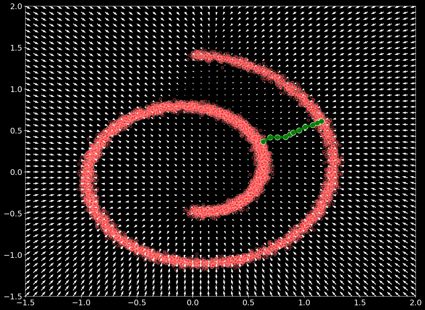
Regarding optimization, we can perform a very simple implementation of this process, by defining ${\mathcal{F}}_{\theta }(\mathbf{x})$ as being any type of neural network. We can perform a minimalistic implementation and observe that our model has learned to represent ${\mathcal{F}}_{\theta }(\mathbf{x})\approx {\nabla }_x\log p(x)$ by plotting the output value across the input space

Sampling

Based on our trained model ${\mathcal{F}}_{\theta }(\mathbf{x})\approx {\nabla }_x\log p(x)$, and using Langevin dynamics, we can produce true samples from a density $p(\mathbf{x})$, by relying only on ${\nabla }_{\mathbf{x}}\log p(\mathbf{x})$, as shown in the following snippet

Diffusion probabilistic models

Diffusion probabilistic models [ 1 ] are based on on a series of latent variables ${\mathbf{x}}_1,\cdots ,{\mathbf{x}}_T$ that have the same dimensionality as a given input data, which is labeled as ${\mathbf{x}}_0\sim q({\mathbf{x}}_0)$. It models two reciprocal processes as Markov chains of these random variables. One (fixed) process $q({\mathbf{x}}_t\mid {\mathbf{x}}_{t-1})$ gradually adds noise to the input data (the diffusion or forward process), destroying the signal up to full noise. Oppositely, the reverse (parametric) process $p_{\theta }({\mathbf{x}}_{t-1}\mid {\mathbf{x}}_t)$ must learn how to denoise local perturbations in order to invert this diffusion process (transform random noise into a high-quality waveform). Hence, learning involves estimating a large number of small perturbations, which is more tractable than trying to directly estimate the full distribution with a single potential function, as examplified in the following figure

Therefore, we need to define the behavior of the two process, and train the reverse process (modeled as conditional Gaussians) using variational inference, which allow for neural network parameterization and tractable estimation.

$$\text{forward (diffusion)}:q({\mathbf{x}}_t\mid {\mathbf{x}}_{t-1})$$ $$\text{reverse (parametric)}:p_{\theta }({\mathbf{x}}_{t-1}\mid {\mathbf{x}}_t)$$

Forward process

In the forward process, the data distribution $q({\mathbf{x}}_0)$ is gradually converted into an analytically tractable distribution $\pi (\mathbf{y})$, by repeated application of a diffusion kernel, so that the complete distribution $q({\mathbf{x}}_{0:T})$ (called diffusion process) is defined as

$$q({\mathbf{x}}_{0:T})=q({\mathbf{x}}_0)\prod _{t=1}^{T}q({\mathbf{x}}_t\mid {\mathbf{x}}_{t-1})$$

This diffusion kernel $q({\mathbf{x}}_t\mid {\mathbf{x}}_{t-1})$ is set to gradually inject Gaussian noise, with a fixed variance schedule ${\beta }_1,\cdots ,{\beta }_T$ such that

$$q({\mathbf{x}}_t\mid {\mathbf{x}}_{t-1})=\mathcal{N}({\mathbf{x}}_t;\sqrt{1-{\beta }_t}{\mathbf{x}}_{t-1},{\beta }_t\mathbf{I})$$

One important property of this forward process noted by Ho et al. [ 1 ] is that we can perform sampling at any arbitrary timestep $t$, such that

$$q({\mathbf{x}}_t\mid {\mathbf{x}}_0)=\mathcal{N}({\mathbf{x}}_t;\sqrt{{\bar{\alpha }}_t}{\mathbf{x}}_0,(1-{\bar{\alpha }}_t)\mathbf{I}),$$

where ${\alpha }_t=1-{\beta }_t$ and ${\bar{\alpha }}_t={\prod }_{s=1}^t{\alpha }_s$. Therefore, we can create a very efficient diffusion sampling function. Note that this depends on the given variance schedule of ${\beta }_1,\cdots ,{\beta }_T$ that we compute prior to the function.

Implementing the forward process

This allows to perform a very efficient implementation of the forward process, where we can directly sample at any given timesteps, as shown in the following code.

Reverse process

The generative distribution that we aim to learn will be trained to perform the reverse trajectory, starting from Gaussian noise to gradually remove local perturbations. Therefore the reverse process starts with our given tractable distribution $p({\mathbf{x}}_T)=\pi ({\mathbf{x}}_T)$ and is described as

$$p_{\theta }({\mathbf{x}}_{0:T})=p({\mathbf{x}}_T)\prod _{t=1}^T{p}_{\theta }({\mathbf{x}}_{t-1}\mid {\mathbf{x}}_t)$$

Each of the transitions in this process can simply be defined as conditional Gaussians (note: which is reminiscent of the definition of VAEs). Therefore, during learning, only the mean and covariancce for a Gaussian diffusion kernel needs to be trained

$$p_{\theta }({\mathbf{x}}_{t-1}\mid {\mathbf{x}}_t)=\mathcal{N}({\mathbf{x}}_{t-1};{\mu }_{\theta }({\mathbf{x}}_t,t),{\mathbf{\Sigma }}_{\theta }({\mathbf{x}}_t,t))$$

The two functions defining the mean ${\mu }_{\theta }({\mathbf{x}}_t,t)$ and covariance ${\mathbf{\Sigma }}_{\theta }({\mathbf{x}}_t,t)$ can be parametrized by deep neural networks. Note also that these functions are parametrized by $t$, which means that a single model can be used for all time steps.

Here, we show a naive implementation of this process, where we have a given model to infer variance. Note that this model is shared across all time steps but conditionned on that said time step.

As we can see, the reverse process consists in inferring the values of the mean and log variance for a given timestep, by providing both the sample ${\mathbf{x}}_t$ at a given time step, and that time step $t$ that we can use to condition the models for ${\mu }_{\theta }({\mathbf{x}}_t,t)$ and ${\mathbf{\Sigma }}_{\theta }({\mathbf{x}}_t,t)$. Finally, obtaining samples from the model is given by running through the whole Markov chain in reverse, starting from a normal distribution to obtain samples from the target distribution. Note that this process can be very slow if we have a large number of steps, as we need to wait for a given ${\mathbf{x}}_t$ to infer the following ${\mathbf{x}}_{t-1}$

Training

By using Jensen's inequality on the previous expression, we can see that the training may be performed by optimizing the variational bound on negative log-likelihood

$$\begin{array}{rl}\mathbb{E}\left[-\log p_{\theta }({\mathbf{x}}_0)\right]& \le {\mathbb{E}}_q\left[-\log \frac{p_{\theta }({\mathbf{x}}_{0:T})}{q({\mathbf{x}}_{1:T}\mid {\mathbf{x}}_0)}\right]\\ \mathcal{L}& ={\mathbb{E}}_q\left[-\log p({\mathbf{x}}_T)-\sum _{t\ge 1}\log \frac{p_{\theta }({\mathbf{x}}_{t-1}\mid {\mathbf{x}}_t)}{q({\mathbf{x}}_t\mid {\mathbf{x}}_{t-1})}\right]\end{array}$$

Therefore, efficient training is allowed by optimizing random terms of $\mathcal{L}$ with gradient descent.

Further improvements, proposed by Ho et al. [ 1 ] , come from variance reduction by rewriting $\mathcal{L}$ as a sum of KL divergences

$$\begin{array}{rl}\mathcal{L}& ={\mathbb{E}}_q\left[{\mathcal{L}}_T+\sum _{t>1}{\mathcal{L}}_{t-1}+{\mathcal{L}}_0\right]\\ {\mathcal{L}}_T& =D_{KL}(q({\mathbf{x}}_T\mid {\mathbf{x}}_0)\Vert p({\mathbf{x}}_T))\\ {\mathcal{L}}_{t-1}& =D_{KL}(q({\mathbf{x}}_{t-1}\mid {\mathbf{x}}_t,{\mathbf{x}}_0)\Vert p_{\theta }({\mathbf{x}}_{t-1}\mid {\mathbf{x}}_t))\\ {\mathcal{L}}_0& =-\log p_{\theta }({\mathbf{x}}_0\mid {\mathbf{x}}_1)\end{array}$$

All the KL divergences defined in this equation compare Gaussians, which means that they have a closed-form solution.

Implementing the loss - random time steps

To optimize this loss, we will need several computational tools, notably the KL divergence between two gaussians, and the entropy of a Gaussian.

The way that the model is trained is slightly counterintuitive, since we select a timestep at random to train for each of the batch input. The implementation taken from the DDIM repo provides a form of antithetic sampling, which allows to ensure that symmetrical points in the different chains are trained jointly. Therefore, the final procedure consists in first run the forward process on each input at a given (random) time steps (performing diffusion). Then we run the reverse process on this sample, and compute the loss.

Denoising diffusion probabilistic models (DDPM)

Ho et al. [ 1 ]  largely enhanced this diffusion models idea, by first proposing to rely on a new parameterization for the mean function $${\mu }_{\theta }({\mathbf{x}}_t,t)=\frac{1}{\sqrt{{\alpha }_t}}\left(({\mathbf{x}}_t-\frac{{\beta }_t}{{\sqrt{1-\bar{\alpha }}}_t}{ϵ}_{\theta }({\mathbf{x}}_t,t)\right)$$

Note that now, the model is trained at directly estimating a form of conditional noise function, which is used in the training and sampling process. Furthermore, the authors suggest to use a fixed variance function

$${\mathbf{x}}_{t-1}=\frac{1}{\sqrt{{\alpha }_t}}\left({\mathbf{x}}_t-\frac{1-{\alpha }_t}{\sqrt{1-\overline{{\alpha }_t}}}{ϵ}_{\theta }({\mathbf{x}}_t,t)\right)+{\sigma }_t\mathbf{z}$$

This leads to a new sampling procedure for the reverse process as follows (we also quickly redefine the model to output the correct dimensionality).

Simplifying loss to denoising score matching

Based on this new parameterization [ 1 ] for the mean of the reverse process $${\mathbf{x}}_{t-1}=\frac{1}{\sqrt{{\alpha }_t}}\left({\mathbf{x}}_t-\frac{1-{\alpha }_t}{\sqrt{1-\overline{{\alpha }_t}}}{ϵ}_{\theta }({\mathbf{x}}_t,t)\right)+{\sigma }_t\mathbf{z}$$ The training objective can simplify to $${\mathcal{L}}_{t-1}-C={\mathbb{E}}_{{\mathbf{x}}_0,ϵ}\left[\frac{{\beta }_t^2}{2{\sigma }_t^2{\alpha }_t(1-{\bar{\alpha }}_t)}\Vert ϵ-{ϵ}_{\theta }(\sqrt{{\bar{\alpha }}_t}{\mathbf{x}}_0+\sqrt{1-{\bar{\alpha }}_t}ϵ,t){\Vert }^2\right]$$ which resembles denoising score matching over multiple noise scales indexed by $t$.

Simplified training objective

The authors proposed to largely simplify the objective, by dropping the initial factor $${\mathcal{L}}_{\text{simple}}={\mathbb{E}}_{t,{\mathbf{x}}_0,ϵ}\left[\Vert ϵ-{ϵ}_{\theta }(\sqrt{{\bar{\alpha }}_t}{\mathbf{x}}_0+\sqrt{1-{\bar{\alpha }}_t}ϵ,t){\Vert }^2\right]$$ They state that this variant is beneficial to the sample quality.

Stabilizing training with Exponential Moving Average (EMA)

This idea is found in most of the implementations, which allows to implement a form of model momentum. Instead of directly updating the weights of the model, we keep a copy of the previous values of the weights, and then update a weighted mean between the previous and new version of the weights. Here, we reuse the implementation proposed in the DDIM repository.

The training loop is finally obtained with the following code

WaveGrad - Applications to waveform generation

Recently, these ideas from score matching and diffusion models were applied to waveform generation, through a model called WaveGrad [ 5 ] . This model proposes a conditional architecture to perform estimation of the gradients of the data log-density. The paper follows almost exactly the training of Ho et al. [ 1 ] , but provides some tricks to ensure the quality of waveform generation.

Toy waveform dataset

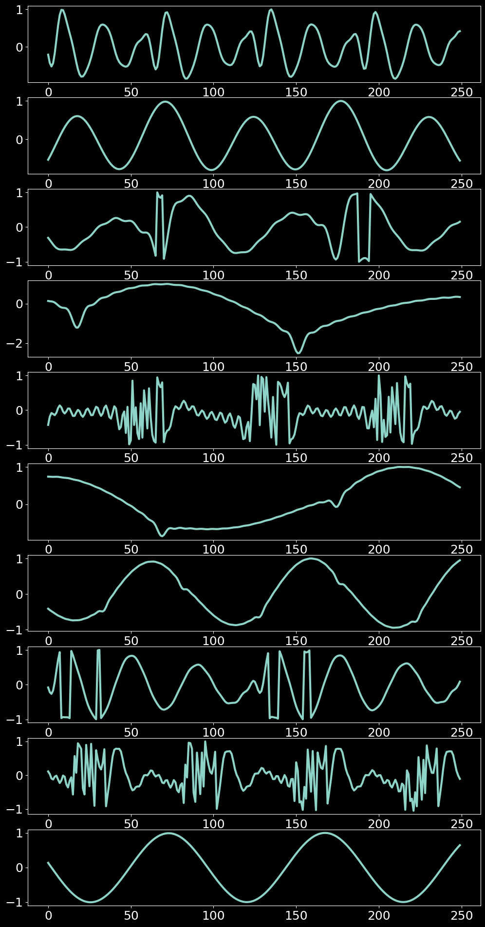
In order to study this model, we will work with a toy dataset of simple waveforms. To do so, we generate a set of random additive sounds as defined in the following function.

WaveGrad model

The WaveGrad model is highly inspired by the DDPM model, but introduces several specificities for training on audio data. First, note that the model is trained to reconstruct a waveform by conditioning on the Mel spectrogram. Hence, this introduces an external conditioning signal , which makes WaveGrad an approach applied to learning conditional generative models of the form $p(\mathbf{y}|\mathbf{x})$. The other major differences introduced by WaveGrad are

1. Conditioning on the continuous noise level (${\beta }_t$), rather than the timestep index ($t$)
2. Fine-tuning the noise schedule (${\beta }_1,\cdots ,{\beta }_T$), depending on the number of steps ($T$)
3. Using a hierarchical sampling scheme on the continuous noise level ($\sqrt{\bar{\alpha }}$)
4. Introducing a specific architecture for waveform generation
   • Using positional encoding (from Transformers)
   • Relying on downsampling and upsampling blocks
   • Using FiLM layers to condition on Mel spectrogram

Introducing a conditional model

Compared to the formulation of DDPM, WaveGrad is defined as a conditional model. This implies that the full model probability is defined as

$$p_{\theta }({\mathbf{x}}_0|\mathbf{y})=\int p_{\theta }({\mathbf{x}}_{0:T}|\mathbf{y})d{\mathbf{x}}_{1:T}$$

where $\mathbf{y}$ is the set of conditioning features (for instance a Mel spectrogram). The forward (diffusion) process remains unchanged, but the reverse (trained) process becomes a condtional definition with

$$p_{\theta }({\mathbf{x}}_{0:T}|\mathbf{y})=p({\mathbf{x}}_T|\mathbf{y})\prod _{t=1}^T{p}_{\theta }({\mathbf{x}}_{t-1}\mid {\mathbf{x}}_t,\mathbf{y})$$

Each of the transitions in this process are still conditional Gaussians, but this time including an extra set of conditioning signal through $\mathbf{y}$. During learning, we still aim to train the mean and covariance for a Gaussian diffusion kernel

$$p_{\theta }({\mathbf{x}}_{t-1}\mid {\mathbf{x}}_t,\mathbf{y})=\mathcal{N}({\mathbf{x}}_{t-1};{\mu }_{\theta }({\mathbf{x}}_t,t,\mathbf{y}),{\mathbf{\Sigma }}_{\theta }({\mathbf{x}}_t,t,\mathbf{y}))$$

Note that in this notebook implementation, we try to avoid using conditioning features and rather aim to directly model the waveform.

Hierarchical sampling scheme - continuous noise level

Similarily to DDPM, the WaveGrad model is trained to infer the noise function, depending on the timestep in the Markov cahin. However, compared to DDPM, the model is now conditioned on the continuous noise level $\sqrt{\overline{{\alpha }_t}}$ instead of the timestep $t$ (and also the extraneous features $\mathbf{y}$). To do so, the model introduces a hierarchical sampling scheme, where we first sample the time step $t$ as $$t\sim \mathcal{U}(\{1,\cdots ,T\})$$ Then, the noise level $\sqrt{\bar{\alpha }}$ is also continuously sampled from a uniform function such that $$\sqrt{\bar{\alpha }}\sim \mathcal{U}(\sqrt{{\bar{\alpha }}_{t-1}},\sqrt{{\bar{\alpha }}_{t-1}}),$$ where ${\bar{\alpha }}_t={\prod }_{s=1}^t{\alpha }_s$ and ${\bar{\alpha }}_t={\prod }_{s=1}^t{\alpha }_s$ where ${\beta }_i$ is a predefined noise schedule (similarly to the original diffusion model definitions).

Therefore, we have to update the sampling function for the forward process, in order to account for this continuous noise sampling scheme.

Impact on the sampling function

ALthough the noise is continuously sampled in the training phase, note that there is no major changes in the sampling (inference) phase. However, we have to update the sampling function as we now need to use the model on a continuous noise level $\sqrt{{\bar{\alpha }}_t}$ rather than the discrete timestep $t$. Note that we also clip the output of the model, so that the sample is contained inside $[-1,1]$.

Loss function

Similarily to DDPM, the WaveGrad model trains on a loss very similar to the denoising score matching objective. This implies that the model tries to infer a form of noise function. However, compared to DDPM, the model is now conditioned on the continuous noise level $\sqrt{\overline{{\alpha }_t}}$ instead of the timestep $t$, and also the extraneous features $\mathbf{y}$. The authors also found that training with the $L_1$ loss instead of the $L_2$ provides a higher quality of samples. This leads to the following loss

$${\mathcal{L}}_{\text{simple}}={\mathbb{E}}_{t,{\mathbf{x}}_0,ϵ}\left[\Vert ϵ-{ϵ}_{\theta }(\sqrt{{\bar{\alpha }}_t}{\mathbf{x}}_0+\sqrt{1-{\bar{\alpha }}_t}ϵ,\mathbf{y},\sqrt{\bar{\alpha }}){\Vert }_1\right],$$

Hence, the implementation is almost identical to that of DDPM, with the continuously sampled noise $\sqrt{\bar{\alpha }}$ and the L1 loss, as shown in the following code

Model architecture

Regarding model architecture, WaveGrad proposes to use several existing mechanisms from the literature in order to solve different parts of the model.

• Using positional encoding (from Transformers)
• Relying on downsampling and upsampling blocks
• Using FiLM layers to condition on Mel spectrogram

As a first approach, we only change the previous model to include the positional encoding, and also add some simple conditional 1-dimensional convolution. This allows to test the overall approach with a simple model wore adapted to waveform data.

Training loop

The training loop with our first simplified architecture is similar to that

Advanced WaveGrad architecture

As discussed earlier, one of the major proposal in the WaveGrad paper concerns the architecture of the model. Notably, we bypassed the specific parts of

• Relying on downsampling and upsampling blocks
• Using FiLM layers to condition on Mel spectrogram

Here, we show the implementation of these blocks for defining the complete WaveGrad model, based on the implementation found in this GitHub

Basic blocks

First the WaveGrad model defines some simple blocks regarding the convolutions and modulation (with FiLM layers).

Bibliography

[1] Ho, J., Jain, A., & Abbeel, P. (2020). Denoising diffusion probabilistic models. arXiv preprint arXiv:2006.11239.
[2] Sohl-Dickstein, J., Weiss, E. A., Maheswaranathan, N., & Ganguli, S. (2015). Deep unsupervised learning using nonequilibrium thermodynamics. arXiv preprint arXiv:1503.03585.
[3] Vincent, P. (2011). A connection between score matching and denoising autoencoders. Neural computation, 23(7), 1661-1674.
[4] Song, J., Meng, C., & Ermon, S. (2020). Denoising Diffusion Implicit Models. arXiv preprint arXiv:2010.02502.
[5] Chen, N., Zhang, Y., Zen, H., Weiss, R. J., Norouzi, M., & Chan, W. (2020). WaveGrad: Estimating gradients for waveform generation. arXiv preprint arXiv:2009.00713.
[6] Hyvärinen, A. (2005). Estimation of non-normalized statistical models by score matching. Journal of Machine Learning Research, 6(Apr), 695-709.
[7] Song, Y., Garg, S., Shi, J., & Ermon, S. (2020, August). Sliced score matching: A scalable approach to density and score estimation. In Uncertainty in Artificial Intelligence (pp. 574-584). PMLR.
[8] Song, Y., & Ermon, S. (2019). Generative modeling by estimating gradients of the data distribution. In Advances in Neural Information Processing Systems (pp. 11918-11930).