


Intro to 4D-STEM data: visualization and analysis with py4DSTEM
Acknowledgements
This tutorial was created by the py4DSTEM instructor team:
- Ben Savitzky (bhsavitzky@lbl.gov)
- Steve Zeltmann (steven.zeltmann@berkeley.edu)
- Stephanie Ribet (sribet@u.northwestern.edu)
- Alex Rakowski (arakowski@lbl.gov)
- Colin Ophus (clophus@lbl.gov)
Last updated:
- Jul 2023 July 17, v0.14.2
Set up the environment
'0.14.3'
Load data
/
|---4DSTEM_simulation
    |---4DSTEM_AuNanoplatelet
    |---4DSTEM_polyAu
    |---defocused_CBED
    |---vacuum_probe
The file we opened holds multiple pieces of data. If we don't specify which data we want, the read function will load all of it. To load only some of the data, we can specify a path within the file to the data we want. For now, we only want the 4D-STEM scan of polycrystalline gold, so we'll specify that with the datapath argument.
What we just did was load data into computer memory and save it as the variable datacube.
Let's take a look at that variable by just passing it directly to the Python interpreter:
DataCube( A 4-dimensional array of shape (100, 84, 125, 125) called '4DSTEM_polyAu',
          with dimensions:

              Rx = [0,1,2,...] pixels
              Ry = [0,1,2,...] pixels
              Qx = [0,1,2,...] pixels
              Qy = [0,1,2,...] pixels
)What's in a DataCube?
This says that datacube is an object of type DataCube. This is py4DSTEM's containter for 4D-STEM scans. We see that it's four-dimensional, with a shape of (100 x 84 x 125 x 125).
What does this mean?
'Real space', or the plane of the sample, has a shape of (100,84), meaning the electron beam was rastered over a 20x20 grid, and
'Diffraction space' or reciprocal space, or the plane of the detector, has a shape of (125,125), meaning the scattered electron intensities are represented in a 125x125 grid.
In py4DSTEM we use 'R' for real space and 'Q' for diffraction space, hence the labels Rx, Ry, Qx, and Qy for the 4 dimensions. Another common convention is to use 'K' for diffraction space.
Currently, we have provided no calibration or pixel sizes to this datacube, which is why the units are in pixels and start at 0 with a step of 1.
(100, 84, 125, 125)
(100, 84, 125, 125)
(100, 84)
(125, 125)
Basic visualization
Evaluating data quality and deciding how to proceed with the analysis almost always begins with visualization. Here, we will go through some visualization functions py4DSTEM uses to visualize 4D data.

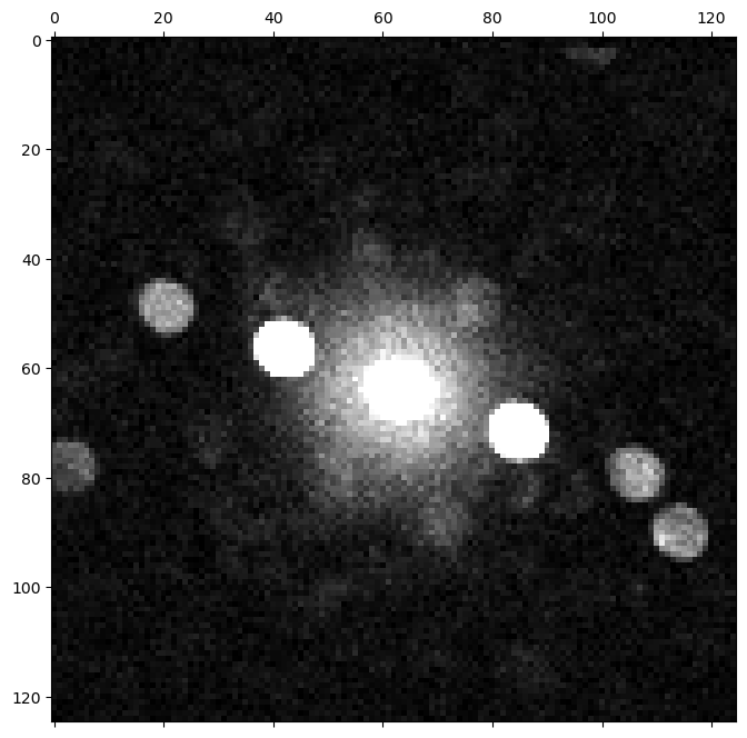

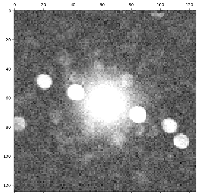
Image scaling and contrast
py4DSTEM tries to automatically set the image contrast in a way that will show many of the image features. However, it is often necessary to modify the scaling and contrast to see as many of the details in the image as possible. We can do this by either using a nonlinear map of intensity --> color, or by adjust the color axis range (or both). We can modify these by adding some additional arguments to the show() function.

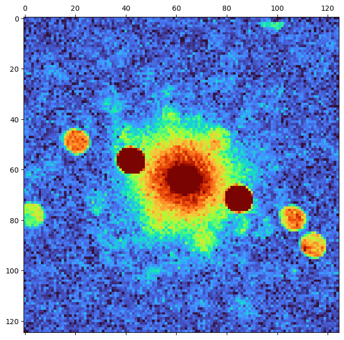
We can see several diffracted Bragg disks, and the distribution of electrons scattered randomly to low angles (characteristic of amorphous samples, or a plasmon background).
However, we had to saturate the center Bragg disk in order to see the weak features. Can we see both strong and weak features?
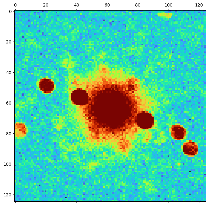
Yes! We just need to use logarithmic or power law scaling of the image intensity.

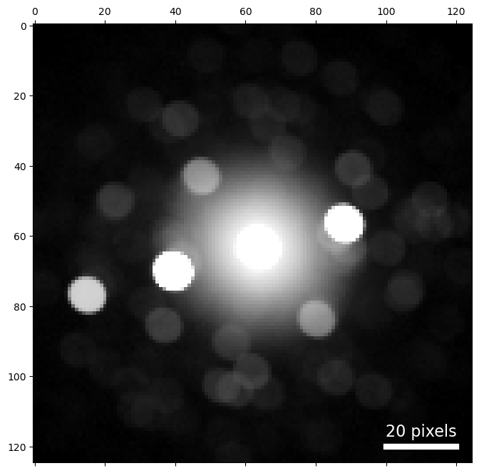
Now we can appreciate the full range of features present in the data:
- the very bright center disk
- somewhat weaker crystalline Bragg diffracted spots
- a small number of electrons randomly scattered to low angles
We can manually specify the intensity range for logarithm scaling too:
Logarithmic scaling is best when the features of interest have intensities which vary by multiple orders of magnitude. It is often a good place to start if you're not sure what to expect in a dataset.
Scaling by a power law is sometimes more useful for visualization of diffraction patterns, because we can tune the power (each pixel intensity --> intensity^power) to achieve the desired scaling. This may exclude some features - and this may be desireable, for instance when extremely weak features are present which are not scientifically interesting or large enough to affect our analysis and which we don't really need to examine closely, such as detector dark current.
Mean and maximum diffraction patterns
The above examples look at a single diffraction pattern. Real experiments might consist of thousands or even millions of diffraction patterns. We want to evaluate the contents of the dataset as quickly as possible - is it single crystal? Polycrstalline? Amorphous? A mixture?
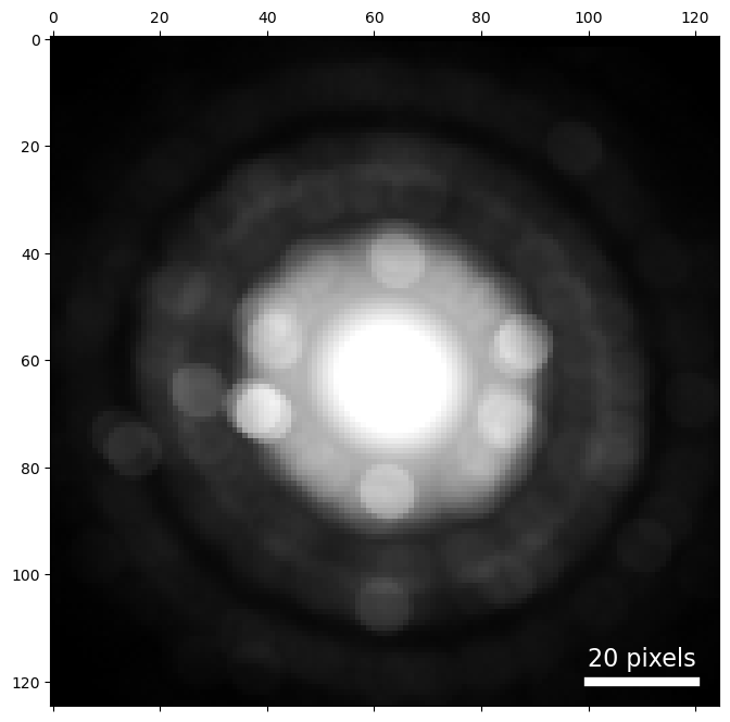
To answer these questions efficiently, it's helpful to get an overview of all of the diffraction that occured in this data acquisition, all at once. The simplest way to do this is to calculate the mean diffraction pattern.
VirtualDiffraction( A 2-dimensional array of shape (125, 125) called 'dp_mean',
                    with dimensions:

                        dim0 = [0,1,2,...] pixels
                        dim1 = [0,1,2,...] pixels
)array([[33.19880952, 33.2647619 , 33.17714286, ..., 32.11107143,
31.93238095, 32.04047619],
[33.18404762, 33.25690476, 33.27964286, ..., 32.08547619,
32.12119048, 32.1022619 ],
[33.2497619 , 33.31821429, 33.35535714, ..., 32.97535714,
32.92845238, 32.96880952],
...,
[33.00154762, 33.20952381, 33.22166667, ..., 33.61547619,
33.51166667, 33.32261905],
[32.96488095, 33.1527381 , 33.12892857, ..., 33.46559524,
33.3802381 , 33.45464286],
[32.88392857, 33.15678571, 33.1697619 , ..., 33.51297619,
33.40535714, 33.43166667]])/ |---dp_mean
VirtualDiffraction( A 2-dimensional array of shape (125, 125) called 'dp_mean',
with dimensions:
dim0 = [0,1,2,...] pixels
dim1 = [0,1,2,...] pixels
)True

We see some interesting features, such as the rings of intensity containing some Bragg disks. However calculating the mean is good and bad: it gives us a quick overview of the most prominent features in many patterns, but it may hide diffraction features which occur in a small number of scan positions.
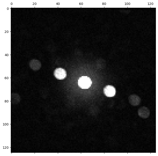
For this reason, we typically also visualize the maximum diffraction pattern. By this, we mean the maximum signal of each pixel in diffraction space over all probe positons. This way, we see the brightest scattering from each pixel, even if it only occured in one diffraction image. This is a great way to see all of the Bragg scattering.
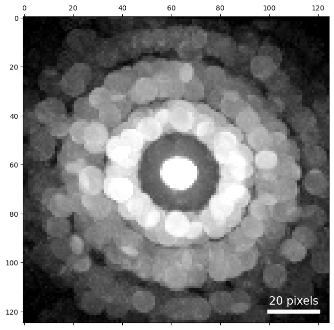
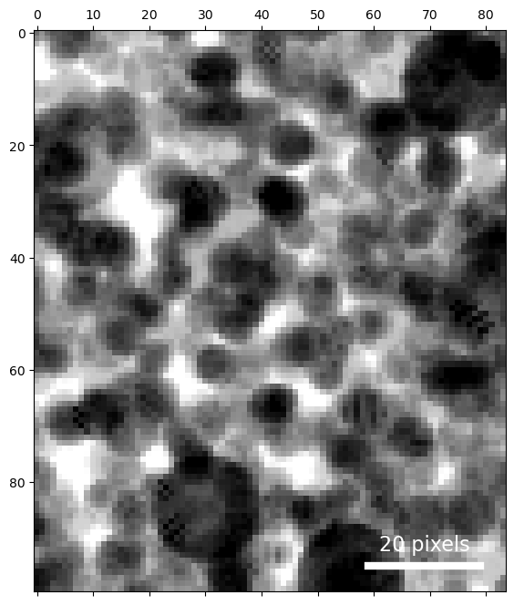
Now we have a good idea of the contents of this 100 x 84 position dataset - various randomly oriented grains with lots of strong Bragg diffraction.
Virtual imaging
Next, let's visualize this data in real space using virtual detectors. We'll generate a virtual bright field (BF) and virtual dark field (DF) image.
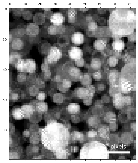
Bright field
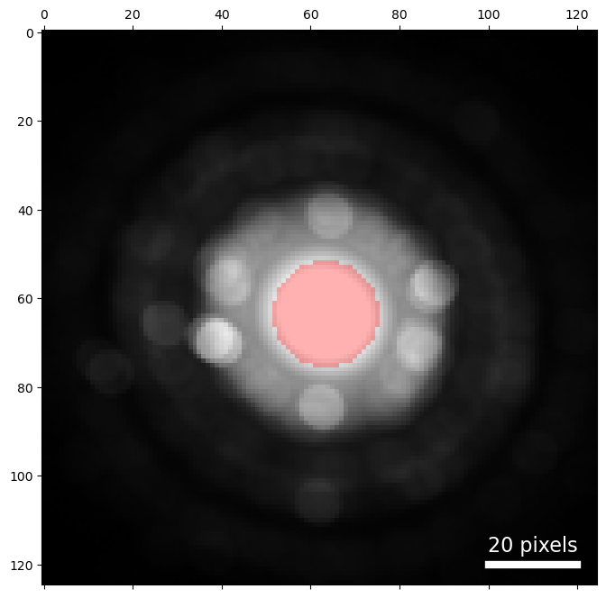
Set detector geometry programmatically
Instead of determining the center and radius by hand, we can do so programmatically by determining the position and radius of the center beam.
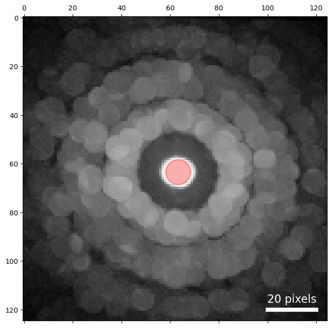
The estimated probe size is slightly too small for our bright-field detector, because of the diffraction shift of this pattern. To compute a bright field image, this radius can be expanded slightly to capture the central disk in all the diffraction images.
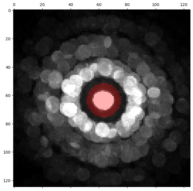
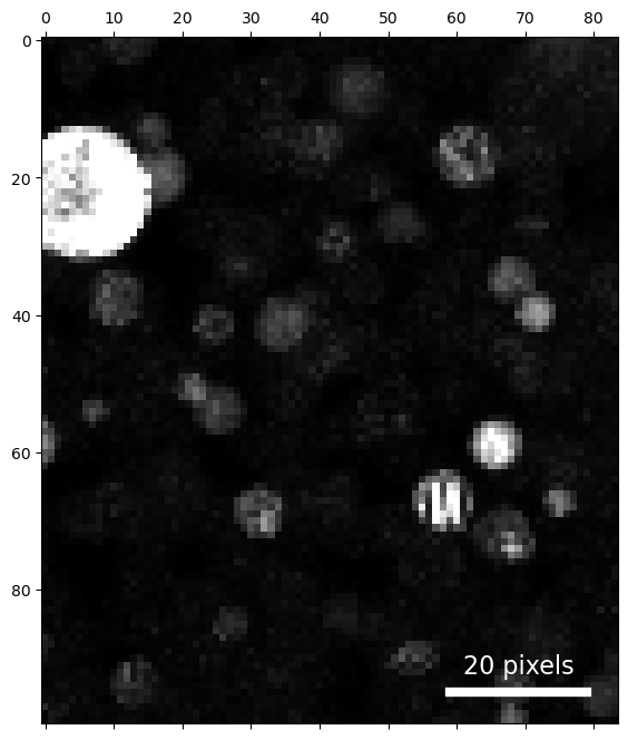
Annular dark-field imaging
For our bright-field image we set the geometry manually. This time, let's use the center and probe size from above.
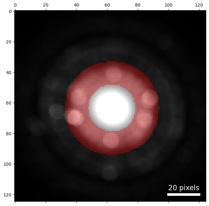
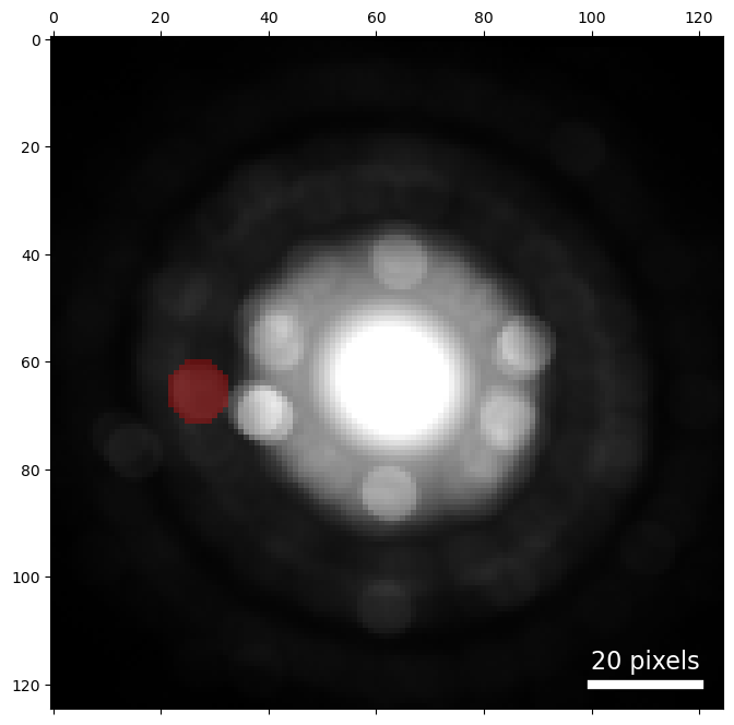
Off axis dark-field imaging
In traditional TEM dark-field imaging, the sample is illuminated with a parallel beam, and an aperture is placed in the diffraction plane around a point of interest, creating pattern in the image plane resulting from electrons scattered only through those areas of diffraction space. We can create an analogous virtual image by placing a circular detector in an off-axis position in diffraction space.
Virtual diffraction
We can also do the inverse - create an average diffraction pattern from some subset of scan positions, showing us what the scattering is like in just those positions in real space.
We've already done a little virtual diffraction - the mean and max diffraction patterns we computed at the beginning of this notebook. In these cases we used all the data; below we'll compute similar patterns using only a selected subset of scan positions.
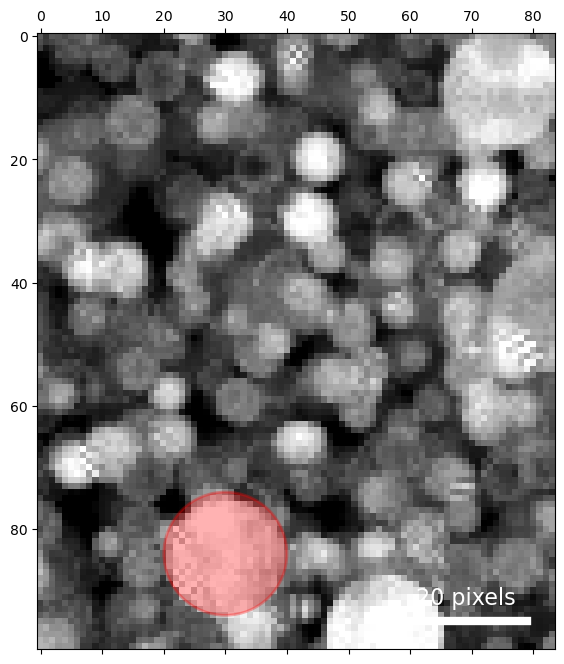
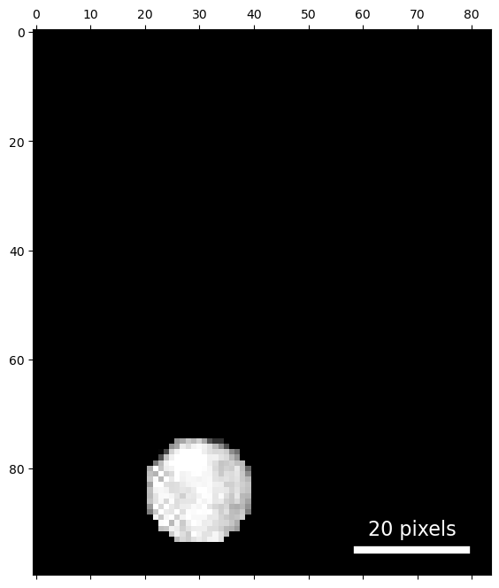
We placed our mask over one Au nanoparticle, so that average diffraction pattern above shows us something about the orientation of this particle. In a later tutorial, we'll see how to map the crystallographic orientations of all the particles in the dataset.
Write and read
'/media/cophus/DataSSD1/4DSTEM/tutorials/analysis_basics_01.h5'
/ |---dp_mean |---dp_max |---bright_field |---annular_dark_field |---virt_dark_field_01 |---selected_area_diffraction_01
/
|---4DSTEM_simulation
    |---annular_dark_field
    |---bright_field
    |---dp_max
    |---dp_mean
    |---selected_area_diffraction_01
    |---virt_dark_field_01
/
|---annular_dark_field
|---bright_field
|---dp_max
|---dp_mean
|---selected_area_diffraction_01
|---virt_dark_field_01
