Random Signals and LTI-Systems

This jupyter notebook is part of a collection of notebooks on various topics of Digital Signal Processing. Please direct questions and suggestions to Sascha.Spors@uni-rostock.de.

Introduction

The response of a system $y[k]=\mathcal{H}\{x[k]\}$ to a random input signal $x[k]$ is the foundation of statistical signal processing. In the following we limit ourselves to linear-time invariant (LTI) systems.

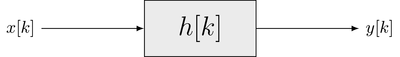
In the following it is assumed that the statistical properties of the input signal $x[k]$ are known. For instance, its first- and second-order ensemble averages. It is further assumed that the impulse response $h[k]$ or the transfer function $H(e^{\mathrm{j}\Omega })$ of the LTI system is given. We are looking for the statistical properties of the output signal $y[k]$ and the joint properties between the input $x[k]$ and output $y[k]$ signal.

Stationarity and Ergodicity

The question arises if the output signal $y[k]$ of an LTI system is (wide-sense) stationary or (wide-sense) ergodic for an input signal $x[k]$ exhibiting the same properties.

Let's assume that the input signal $x[k]$ is drawn from a stationary random process. According to the definition of stationarity the following relation must hold

$$\begin{array}{c}E\{f(x[k_1],x[k_2],\dots )\}=E\{f(x[k_1+\Delta ],x[k_2+\Delta ],\dots )\}\end{array}$$

where $\Delta \in \mathbb{Z}$ denotes an arbitrary (temporal) shift and $f(\cdot )$ an arbitary mapping function. The condition for time-invariance of a system reads

$$\begin{array}{c}y[k+\Delta ]=\mathcal{H}\{x[k+\Delta ]\}\end{array}$$

for $y[k]=\mathcal{H}\{x[k]\}$. Applying the system operator $\mathcal{H}\{\cdot \}$ to the left- and right-hand side of the definition of stationarity for the input signal $x[k]$ and recalling the linearity of the expectation operator $E\{\cdot \}$ yields

$$\begin{array}{c}E\{g(y[k_1],y[k_2],\dots )\}=E\{g(y[k_1+\Delta ],y[k_2+\Delta ],\dots )\}\end{array}$$

where $g(\cdot )$ denotes an arbitrary mapping function that may differ from $f(\cdot )$. From the equation above, it can be concluded that the output signal of an LTI system for a stationary input signal is also stationary. The same reasoning can also be applied to an ergodic input signal. Since both wide-sense stationarity (WSS) and wide-sense ergodicity are special cases of the general case, the derived results hold also here.

Summarizing, for an input signal $x[k]$ that is

• (wide-sense) stationary, the output signal $y[k]$ is (wide-sense) stationary and the in- and output is jointly (wide-sense) stationary
• (wide-sense) ergodic, the output signal $y[k]$ is (wide-sense) ergodic and the in- and output is jointly (wide-sense) ergodic

This implies for instance, that for a WSS input signal $x[k]$ measures like the auto-correlation function (ACF) can also be applied to the output signal $y[k]=\mathcal{H}\{x[k]\}$ of an LTI system.

Example - Response of an LTI system to a random signal

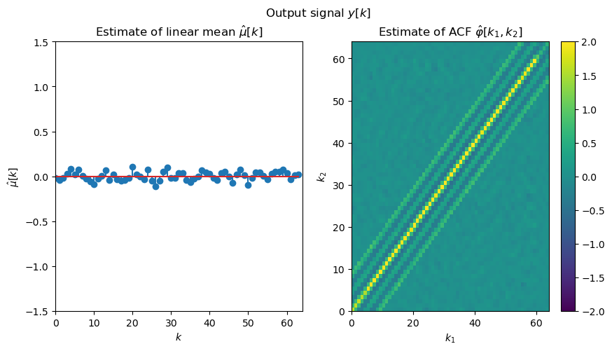
The following example computes and plots estimates of the linear mean $\mu [k]$ and auto-correlation function (ACF) $\phi [k_1,k_2]$ for the in- and output of an LTI system. The input $x[k]$ is drawn from a normally distributed white noise process.

Exercise

• Are the in- and output signals WSS?
• Can the output signal $y[k]$ be assumed to be white noise?

Solution: From the shown results it can assumed for the input signal $x[k]$ that the linear mean ${\mu }_x[k]$ does not depend on the time-index $k$ and that the ACF ${\phi }_{xx}[k_1,k_2]$ does only depend on the difference $\kappa =k_1-k_2$ of both time indexes. The same holds also for the output signal $y[k]$. Hence both the in- and output signal are WSS. Although the input signal $x[k]$ can be assumed to be white noise, the output signal $y[k]$ is not white noise due to its ACF ${\phi }_{yy}[k_1,k_2]$.

Copyright

This notebook is provided as Open Educational Resource. Feel free to use the notebook for your own purposes. The text is licensed under Creative Commons Attribution 4.0, the code of the IPython examples under the MIT license. Please attribute the work as follows: Sascha Spors, Digital Signal Processing - Lecture notes featuring computational examples.