Random Signals and LTI-Systems

This jupyter notebook is part of a collection of notebooks on various topics of Digital Signal Processing. Please direct questions and suggestions to Sascha.Spors@uni-rostock.de.

Auto-Correlation Function

The auto-correlation function (ACF) ${\phi }_{yy}[\kappa ]$ of the output signal of an LTI system $y[k]=\mathcal{H}\{x[k]\}$ is derived. It is assumed that the input signal is a wide-sense stationary (WSS) real-valued random process and that the LTI system has a real-valued impulse repsonse $h[k]\in \mathbb{R}$.

Introducing the output relation $y[k]=h[k]\ast x[k]$ of an LTI system into the definition of the ACF and rearranging terms yields

$$\begin{array}{c}\begin{array}{rl}{\phi }_{yy}[\kappa ]& =E\{y[k+\kappa ]\cdot y[k]\}\\ & =E\left\{\sum _{\mu =-\infty }^{\infty }h[\mu ]x[k+\kappa -\mu ]\cdot \sum _{\nu =-\infty }^{\infty }h[\nu ]x[k-\nu ]\right\}\\ & =\underset{{\phi }_{hh}[\kappa ]}{\underbrace{h[\kappa ]\ast h[-\kappa ]}}\ast {\phi }_{xx}[\kappa ]\end{array}\end{array}$$

where the ACF ${\phi }_{hh}[\kappa ]$ of the deterministic impulse response $h[k]$ is commonly termed as filter ACF. This is related to the link between ACF and convolution. The relation above is known as the Wiener-Lee theorem. It states that the ACF of the output ${\phi }_{yy}[\kappa ]$ of an LTI system is given by the convolution of the input signal's ACF ${\phi }_{xx}[\kappa ]$ with the filter ACF ${\phi }_{hh}[\kappa ]$. For a system which just attenuates the input signal $y[k]=A\cdot x[k]$ with $A\in \mathbb{R}$, the ACF at the output is given as ${\phi }_{yy}[\kappa ]=A^2\cdot {\phi }_{xx}[\kappa ]$.

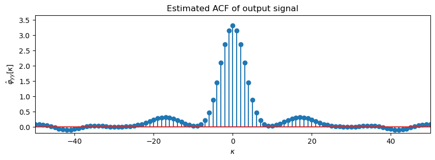
Example - System Response to White Noise

Let's assume that the wide-sense ergodic input signal $x[k]$ of an LTI system with impulse response $h[k]={\text{rect}}_N[k]$ is normal distributed white noise. Introducing ${\phi }_{xx}[\kappa ]=N_0\delta [\kappa ]$ and $h[k]$ into the Wiener-Lee theorem yields

$$\begin{array}{c}{\phi }_{yy}[\kappa ]=N_0\cdot {\phi }_{hh}[\kappa ]=N_0\cdot ({\text{rect}}_N[\kappa ]\ast {\text{rect}}_N[-\kappa ])\end{array}$$

The example is evaluated numerically for $N_0=1$ and $N=5$

Exercise

• Derive the theoretic result for ${\phi }_{yy}[\kappa ]$ by calculating the filter-ACF ${\phi }_{hh}[\kappa ]$.
• Why is the estimated ACF ${\hat{\phi }}_{yy}[\kappa ]$ of the output signal not exactly equal to its theoretic result ${\phi }_{yy}[\kappa ]$?
• Change the number of samples L and rerun the example. What changes?

Solution: The filter-ACF is given by ${\phi }_{hh}[\kappa ]={\text{rect}}_N[\kappa ]\ast {\text{rect}}_N[-\kappa ]$. The convolution of two rectangular signals ${\text{rect}}_N[\kappa ]$ results in a triangular signal. Taking the time reversal into account yields

$$\begin{array}{c}{\phi }_{hh}[\kappa ]=\{\begin{array}{ll}N-|\kappa |& \text{for }-N<\kappa \le N\\ 0& \text{otherwise}\end{array}\end{array}$$

for even $N$. The estimated ACF ${\hat{\phi }}_{yy}[\kappa ]$ differs from its theoretic value due to the statistical uncertainties when using random signals of finite length. Increasing its length L lowers the statistical uncertainties.

Cross-Correlation Function

The cross-correlation functions (CCFs) ${\phi }_{xy}[\kappa ]$ and ${\phi }_{yx}[\kappa ]$ between the in- and output signal of an LTI system $y[k]=\mathcal{H}\{x[k]\}$ are derived. As for the ACF it is assumed that the input signal originates from a wide-sense stationary real-valued random process and that the LTI system's impulse response is real-valued, i.e. $h[k]\in \mathbb{R}$.

Introducing the convolution into the definition of the CCF and rearranging the terms yields

$$\begin{array}{c}\begin{array}{rl}{\phi }_{xy}[\kappa ]& =E\{x[k+\kappa ]\cdot y[k]\}\\ & =E\left\{x[k+\kappa ]\cdot \sum _{\mu =-\infty }^{\infty }h[\mu ]x[k-\mu ]\right\}\\ & =\sum _{\mu =-\infty }^{\infty }h[\mu ]\cdot E\{x[k+\kappa ]\cdot x[k-\mu ]\}\\ & =h[-\kappa ]\ast {\phi }_{xx}[\kappa ]\end{array}\end{array}$$

The CCF ${\phi }_{xy}[\kappa ]$ between in- and output is given as the time-reversed impulse response of the system convolved with the ACF of the input signal.

The CCF between out- and input is yielded by taking the symmetry relations of the CCF and ACF into account

$$\begin{array}{c}{\phi }_{yx}[\kappa ]={\phi }_{xy}[-\kappa ]=h[\kappa ]\ast {\phi }_{xx}[\kappa ]\end{array}$$

The CCF ${\phi }_{yx}[\kappa ]$ between out- and input is given as the impulse response of the system convolved with the ACF of the input signal.

For a system which just attenuates the input signal $y[k]=A\cdot x[k]$, the CCFs between input and output are given as ${\phi }_{xy}[\kappa ]=A\cdot {\phi }_{xx}[\kappa ]$ and ${\phi }_{yx}[\kappa ]=A\cdot {\phi }_{xx}[\kappa ]$.

System Identification by Cross-Correlation

The process of determining the impulse response or transfer function of a system is referred to as system identification. The CCFs of an LTI system play an important role in the estimation of the impulse response $h[k]$ of an unknown system. This is illustrated in the following.

The basic idea is to use a specific measurement signal as input signal to the system. Let's assume that the unknown LTI system is excited by white noise. The ACF of the wide-sense stationary input signal $x[k]$ is then given as ${\phi }_{xx}[\kappa ]=N_0\cdot \delta [\kappa ]$. According to the relation derived above, the CCF between out- and input for this special choice of the input signal becomes

$$\begin{array}{c}{\phi }_{yx}[\kappa ]=h[\kappa ]\ast N_0\cdot \delta [\kappa ]=N_0\cdot h[\kappa ]\end{array}$$

For white noise as input signal $x[k]$, the impulse response of an LTI system can be estimated by estimating the CCF between its out- and input signals. Using noise as measurement signal instead of a Dirac impulse is beneficial since its crest factor is limited.

Example

The application of the CCF to the identification of a system is demonstrated. The system is excited by wide-sense ergodic normal distributed white noise with $N_0=1$. The ACF of the in- and output, as well as the CCF between out- and input is estimated and plotted.

Exercise

• Why is the estimated CCF ${\hat{\phi }}_{yx}[k]$ not exactly equal to the true impulse response $h[k]$ of the system?
• What changes if you change the number of samples N of the input signal?

Solution: The derived relations for system identification hold for the case of a wide-sense ergodic input signal of infinite duration. Since we can only numerically simulate signals of finite duration, the observed deviations are a result of the resulting statistical uncertainties. Increasing the length N of the input signal improves the estimate of the impulse response.

Copyright

This notebook is provided as Open Educational Resource. Feel free to use the notebook for your own purposes. The text is licensed under Creative Commons Attribution 4.0, the code of the IPython examples under the MIT license. Please attribute the work as follows: Sascha Spors, Digital Signal Processing - Lecture notes featuring computational examples.