Random Signals and LTI-Systems

This jupyter notebook is part of a collection of notebooks on various topics of Digital Signal Processing. Please direct questions and suggestions to Sascha.Spors@uni-rostock.de.

The Wiener Filter

The Wiener filter, named after Norbert Wiener, aims at estimating an unknown random signal by filtering a noisy distorted observation of the signal. It has a wide range of applications in signal processing. For instance, noise reduction, system identification, deconvolution and signal detection. The Wiener filter is frequently used as basic building block for algorithms that denoise audio signals, like speech, or remove noise from a image.

Signal Model

The following signal model is underlying the Wiener filter

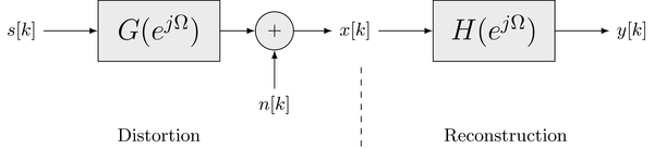
The random signal $s[k]$ is subject to distortion by the linear time-invariant (LTI) system $G({\mathrm{e}}^{\mathrm{j}\Omega })$ and additive noise $n[k]$, resulting in the observed signal $x[k]=s[k]\ast g[k]+n[k]$. The additive noise $n[k]$ is assumed to be uncorrelated from $s[k]$. It is furthermore assumed that all random signals are wide-sense stationary (WSS). This distortion model holds for many practical problems, like e.g. the measurement of a physical quantity by a sensor.

The basic concept of the Wiener filter is to apply the LTI system $H({\mathrm{e}}^{\mathrm{j}\Omega })$ to the observed signal $x[k]$ such that the output signal $y[k]=x[k]\ast h[k]$ matches $s[k]$ as close as possible. In order to quantify the deviation between $y[k]$ and $s[k]$, the error signal

$$\begin{array}{c}e[k]=y[k]-s[k]\end{array}$$

is introduced. The error $e[k]$ equals zero, if the output signal $y[k]$ perfectly matches $s[k]$. In general, this goal cannot be achieved in a strict sense. As alternative one could aim at minimizing the linear average of the error $e[k]$. However, this quantity is not very well suited for optimization since it is signed. Instead, the quadratic average of the error $e[k]$ is used in the Wiener filter and other techniques. This measure is known as mean squared error (MSE). It is defined as

$$\begin{array}{c}E\{|e[k]{|}^2\}=\frac{1}{2\pi }\underset{-\pi }{\overset{\pi }{\int }}{\Phi }_{ee}({\mathrm{e}}^{\mathrm{j}\Omega })\mathrm{d}\Omega ={\phi }_{ee}[\kappa ]{|}_{\kappa =0}\end{array}$$

the equalities are deduced from the properties of the power spectral density (PSD) and the auto-correlation function (ACF). Above equation is referred to as cost function. We aim at minimizing the cost function, hence minimizing the MSE between the original signal $s[k]$ and its estimate $y[k]$. The solution is referred to as minimum mean squared error (MMSE) solution.

Transfer Function of the Wiener Filter

At first, the Wiener filter shall only have access to the observed signal $x[k]$ and selected statistical measures. It is assumed that the cross-power spectral density ${\Phi }_{xs}({\mathrm{e}}^{\mathrm{j}\Omega })$ between the observed signal $x[k]$ and the original signal $s[k]$, and the PSD of the observed signal ${\Phi }_{xx}({\mathrm{e}}^{\mathrm{j}\Omega })$ are known. This knowledge can either be gained by estimating both from measurements taken at an actual system or by using suitable statistical models.

The optimal filter is found by minimizing the MSE $E\{|e[k]{|}^2\}$ with respect to the transfer function $H({\mathrm{e}}^{\mathrm{j}\Omega })$. The solution of this optimization problem goes beyond the scope of this notebook and can be found in the literature, e.g. [Girod et. al]. The transfer function of the Wiener filter is given as

$$\begin{array}{c}H({\mathrm{e}}^{\mathrm{j}\Omega })=\frac{{\Phi }_{sx}({\mathrm{e}}^{\mathrm{j}\Omega })}{{\Phi }_{xx}({\mathrm{e}}^{\mathrm{j}\Omega })}=\frac{{\Phi }_{xs}({\mathrm{e}}^{-\mathrm{j}\Omega })}{{\Phi }_{xx}({\mathrm{e}}^{\mathrm{j}\Omega })}\end{array}$$

for ${\Phi }_{xx}({\mathrm{e}}^{\mathrm{j}\Omega })\ne 0$. No knowledge on the actual distortion process is required besides the assumption of an LTI system and additive noise. Only the PSDs ${\Phi }_{sx}({\mathrm{e}}^{\mathrm{j}\Omega })$ and ${\Phi }_{xx}({\mathrm{e}}^{\mathrm{j}\Omega })$ have to be known in order to estimate $s[k]$ from $x[k]$ in the MMSE sense. Care has to be taken that the filter $H({\mathrm{e}}^{\mathrm{j}\Omega })$ is causal and stable in practical applications.

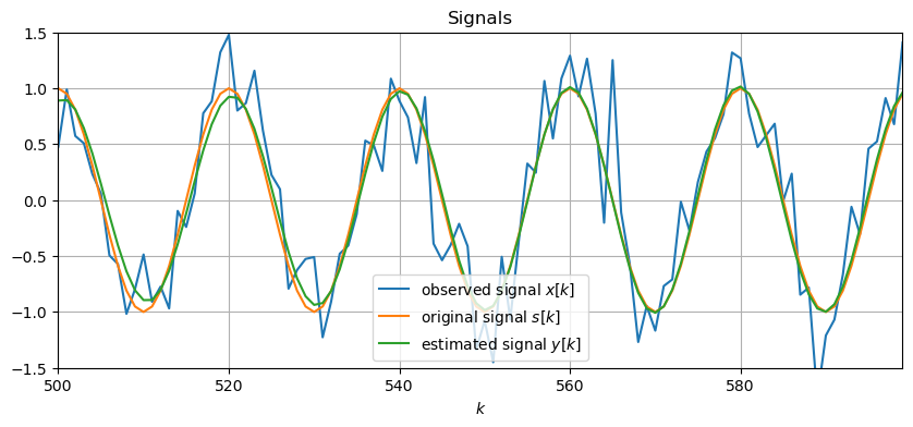
Example - Denoising of an Deterministic Signal

The following example considers the estimation of the original signal from a distorted observation. It is assumed that the original signal is a deterministic signal $s[k]=\sin [{\Omega }_{0}k]$ which is distorted by an LTI system and additive wide-sense ergodic normal distributed zero-mean white noise with PSD $N_0=0.1$. The PSDs ${\Phi }_{sx}({\mathrm{e}}^{\mathrm{j}\Omega })$ and ${\Phi }_{xx}({\mathrm{e}}^{\mathrm{j}\Omega })$ are estimated from $s[k]$ and $x[k]$ using the Welch technique. The Wiener filter is applied to the observation $x[k]$ in order to compute the estimate $y[k]$ of $s[k]$. Note that the discrete signals have been illustrated by continuous lines for ease of illustration.

Let's listen to the observed signal $x[k]$ and the output of the Wiener filter $y[k]$

Observed signal

./Wiener_observed_signal.wav

Output of Wiener filter

./Wiener_output.wav

Exercise

• Take a look at the PSDs and the resulting transfer function of the Wiener filter. How does the Wiener filter remove the noise from the observed signal?
• Change the frequency Om0 of the original signal $s[k]$ and the noise power N0 of the additive noise. What changes?

Solution: The cross-PSD ${\Phi }_{sx}(e^{j\Omega })$ has its maximum at the frequency ${\Omega }_0$ of the original signal $s[k]$, besides this frequency the PSD ${\Phi }_{xx}(e^{j\Omega })$ has approximately the value of the PSD ${\Phi }_{nn}(e^{j\Omega })=N_0$ of the additive noise. The resulting Wiener filter $G(e^{j\Omega })$ has an attenuation of 0 dB at ${\Omega }_0$ which increases off this frequency. It has the characteristics of a band-pass filter centered at ${\Omega }_0$. By filtering the observed signal $x[k]$ with the Wiener filter, the major portion of the additive white noise is removed. However, around ${\Omega }_0$ both the original signal $s[k]$ and noise pass the filter. This explains the remaining small deviations between the estimated signal $y[k]$ and the original signal $y[k]$. The adaption of the Wiener filter to the original signal and additive noise changes when changing its frequency and PSD.

Wiener Deconvolution

As discussed above, the general formulation of the Wiener filter is based on the knowledge of the PSDs ${\Phi }_{sx}({\mathrm{e}}^{\mathrm{j}\Omega })$ and ${\Phi }_{xx}({\mathrm{e}}^{\mathrm{j}\Omega })$ characterizing the distortion process and the observed signal, respectively. These PSDs can be derived from the PSDs of the original signal ${\Phi }_{ss}({\mathrm{e}}^{\mathrm{j}\Omega })$ and the noise ${\Phi }_{nn}({\mathrm{e}}^{\mathrm{j}\Omega })$, and the transfer function $G({\mathrm{e}}^{\mathrm{j}\Omega })$ of the distorting system.

Under the assumption that $n[k]$ is uncorrelated from $s[k]$, the PSD ${\Phi }_{sx}({\mathrm{e}}^{\mathrm{j}\Omega })$ can be derived as

$$\begin{array}{c}{\Phi }_{sx}({\mathrm{e}}^{\mathrm{j}\Omega })={\Phi }_{ss}({\mathrm{e}}^{\mathrm{j}\Omega })\cdot G({\mathrm{e}}^{-\mathrm{j}\Omega })\end{array}$$

and

$$\begin{array}{c}{\Phi }_{xx}({\mathrm{e}}^{\mathrm{j}\Omega })={\Phi }_{ss}({\mathrm{e}}^{\mathrm{j}\Omega })\cdot |G({\mathrm{e}}^{\mathrm{j}\Omega }){|}^2+{\Phi }_{nn}({\mathrm{e}}^{\mathrm{j}\Omega })\end{array}$$

Introducing these results into the general formulation of the Wiener filter yields

$$\begin{array}{c}H({\mathrm{e}}^{\mathrm{j}\Omega })=\frac{{\Phi }_{ss}({\mathrm{e}}^{\mathrm{j}\Omega })\cdot G({\mathrm{e}}^{-\mathrm{j}\Omega })}{{\Phi }_{ss}({\mathrm{e}}^{\mathrm{j}\Omega })\cdot |G({\mathrm{e}}^{\mathrm{j}\Omega }){|}^2+{\Phi }_{nn}({\mathrm{e}}^{\mathrm{j}\Omega })}\end{array}$$

This specialization is also known as Wiener deconvolution filter. The filter can be derived from the PSDs of the original signal $s[k]$ and the noise $n[k]$, and the transfer function $G({\mathrm{e}}^{\mathrm{j}\Omega })$ of the distorting system. This form is especially useful when the PSDs can be modeled reasonably well by analytic probabilty density functions (PSDs). In many cases, the additive noise can be modeled as white noise ${\Phi }_{nn}(e^{j\Omega })=N_0$.

Interpretation

The Wiener deconvolution filter derived above is also useful for an interpretation of the operation of the Wiener filter. It can be rewritten by introducing the frequency dependent signal-to-noise ratio $\text{SNR}({\mathrm{e}}^{\mathrm{j}\Omega })=\frac{{\Phi }_{ss}({\mathrm{e}}^{\mathrm{j}\Omega })}{{\Phi }_{nn}({\mathrm{e}}^{\mathrm{j}\Omega })}$ between the original signal and the noise as

$$\begin{array}{c}H({\mathrm{e}}^{\mathrm{j}\Omega })=\frac{1}{G({\mathrm{e}}^{\mathrm{j}\Omega })}\cdot \left(\frac{|G({\mathrm{e}}^{\mathrm{j}\Omega }){|}^2}{|G({\mathrm{e}}^{\mathrm{j}\Omega }){|}^2+\frac{1}{\text{SNR}({\mathrm{e}}^{\mathrm{j}\Omega })}}\right)\end{array}$$

Now two special cases are discussed:

1. If there is no additive noise ${\Phi }_{nn}({\mathrm{e}}^{\mathrm{j}\Omega })=0$, the bracketed expression is equal to 1. Hence, the Wiener filter is simply given as the inverse system to the distorting system $$H({\mathrm{e}}^{\mathrm{j}\Omega })=\frac{1}{G({\mathrm{e}}^{\mathrm{j}\Omega })}$$

2. If the distorting system is just a pass-through $G({\mathrm{e}}^{\mathrm{j}\Omega })=1$, the Wiener filter is given as

   $$H({\mathrm{e}}^{\mathrm{j}\Omega })=\frac{\text{SNR}({\mathrm{e}}^{\mathrm{j}\Omega })}{\text{SNR}({\mathrm{e}}^{\mathrm{j}\Omega })+1}=\frac{{\Phi }_{ss}({\mathrm{e}}^{\mathrm{j}\Omega })}{{\Phi }_{ss}({\mathrm{e}}^{\mathrm{j}\Omega })+{\Phi }_{nn}({\mathrm{e}}^{\mathrm{j}\Omega })}$$ Two extreme cases are considered

   • for ${\Phi }_{ss}({\mathrm{e}}^{\mathrm{j}\Omega })\gg {\Phi }_{nn}({\mathrm{e}}^{\mathrm{j}\Omega })$ (high $\text{SNR}({\mathrm{e}}^{\mathrm{j}\Omega })$) at a given frequency $\Omega$ the transfer function approaches 1
   • for ${\Phi }_{ss}({\mathrm{e}}^{\mathrm{j}\Omega })\ll {\Phi }_{nn}({\mathrm{e}}^{\mathrm{j}\Omega })$ (low $\text{SNR}({\mathrm{e}}^{\mathrm{j}\Omega })$) at a given frequency $\Omega$ the transfer function approaches 0

The discussed cases explain the operation of the Wiener filter for specific situations, the general operation is a combination of these.

Example - Denoising of a deterministic signal with the Wiener deconvolution filter

The preceding example of the general Wiener filter will now be reevaluated with the Wiener deconvolution filter.

Exercise

• Compare the transfer function of the Wiener deconvolution filter to the transfer function of the general Wiener filter from the preceding example.
• What is different compared to the general Wiener filter? Why?

Solution: The transfer function $H(e^{j\Omega })$ of the Wiener deconvolution filter is much smoother than the transfer function of the general Wiener filter from the preceding example. This is due to the knowledge of the transfer function $G(e^{j\Omega })$ of the disturbing system. The general Wiener filter inherently estimates this from the noisy observations.

Copyright

This notebook is provided as Open Educational Resource. Feel free to use the notebook for your own purposes. The text is licensed under Creative Commons Attribution 4.0, the code of the IPython examples under the MIT license. Please attribute the work as follows: Sascha Spors, Digital Signal Processing - Lecture notes featuring computational examples.