空间站广场

论文

Notebooks

比赛

课程

Apps

我的主页

我的Notebooks

我的论文库

我的足迹

我的工作空间

任务

节点

文件

数据集

镜像

项目

数据库

公开

使用DMFF进行液体碳酸二甲酯（DMC）的力场优化

DMFF

分子动力学

DMFFMD分子动力学

Feng Wei

yuk@dp.tech

发布于 2023-09-26

推荐镜像 :Third-party software:dmff:0.2.0-notebook

推荐机型 :c2_m4_cpu

使用DMFF进行液体碳酸二甲酯（DMC）的力场优化

1. 介绍

2. 安装环境依赖

3. 定义势函数

4. 定义OpenMM采样器：

5. 初始MD采样

6. 定义性质计算函数

7. 读入数据并进行比对

8. Estimator 初始化

9. 定义目标系综

10. 定义损失函数

11. 优化器准备以及优化循环

使用DMFF进行液体碳酸二甲酯（DMC）的力场优化

reporter：冯维

代码

文本

1. 介绍

用DMFF搭建工作流的初始步骤是产生势函数，其流程和API与OpenMM类似，大致如下：

首先定义力场对象（DMFF中称之为Hamiltonian），其中定义了原子归类（typification）规则以及所有的力场参数。大体上相当于表达为python对象的openmm的xml文件或是gromacs的itp文件。
获取所需要模拟的体系的分子键连拓扑信息（通过pdb文件得到）。
根据体系的连接拓扑，使用Hamiltonian对其中的每个原子、键长、键角、二面角等进行归类并参数化，创建势函数。势函数一般以原子位置、盒子大小、力场参数为输入，方便后续求导运算。
如有必要，对势函数进行必要的修饰和拓展。例如，利用jax.grad得到力、维里矩阵的计算函数，可以直接用于MD模拟。
也可以利用势函数定义相应性质的estimator和损失函数，并利用梯度下降优化器进行相应的参数优化。

在DMFF中，我们提供了传统物理力场中PME、对相互作用、多极矩、可极化力场等势函数的JAX实现。利用JAX提供的修饰工具，用户可以对这些势函数进行微分，向量化、编译等修饰，也可以对其进行再封装和重组合以实现新的势函数，也可以基于这些势函数开发性质估计函数（property estimators），而这些新的函数也可以进一步被求导或者向量化。可以看出，这种以函数变换为核心的编程范式为DMFF中新力场、新目标函数的定义提供了无与伦比的灵活性。

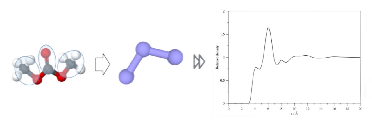
接下来，为了用户对DMFF中的主要模块和功能有个全面的认识，展示这些模块在力场开发中是如何互相配合的，我们通过碳酸二甲酯（DMC）的粗粒化模型，演示在DMFF中一个模型从定义、优化、到部署的全过程。任务的目标是：使用三个site表示DMC长链（以下称为3-site模型），如何优化这三个site间的相互作用，复现XRD实验测出的液体DMC的径向分布函数（Radial Distribution Function, RDF）并将DMC粗粒化模型力场与全原子模型OPLS-AA力场进行比对。

代码

文本

代码

文本

2. 安装环境依赖

代码

文本

[1]

#! pip install matplotlib pymbar optax

#! conda install mdtraj -y

! if [ ! -e DMFF ];then git clone https://gitee.com/deepmodeling/DMFF.git;fi

! git config --global --add safe.directory `pwd`/DMFF

! cd DMFF && git checkout devel

! export XLA_PYTHON_CLIENT_PREALLOCATE=FALSE

#! cd DMFF && python setup.py install

Cloning into 'DMFF'...
remote: Enumerating objects: 3233, done.
remote: Counting objects: 100% (3233/3233), done.
remote: Compressing objects: 100% (1726/1726), done.
remote: Total 3233 (delta 2119), reused 2243 (delta 1435), pack-reused 0
Receiving objects: 100% (3233/3233), 17.93 MiB | 1.90 MiB/s, done.
Resolving deltas: 100% (2119/2119), done.
Updating files: 100% (273/273), done.
Branch 'devel' set up to track remote branch 'devel' from 'origin'.
Switched to a new branch 'devel'

代码

文本

[2]

import os

os.chdir(os.path.join("DMFF","examples", "DMC"))

代码

文本

3. 定义势函数

代码

文本

[3]

import sys

import numpy as np

import openmm as mm

import openmm.app as app

import openmm.unit as unit

import numpy as np

import mdtraj as md

from dmff.mbar import MBAREstimator, SampleState, TargetState, Sample, OpenMMSampleState, buildTrajEnergyFunction

from dmff.optimize import MultiTransform, genOptimizer

from dmff import Hamiltonian, NeighborListFreud

import jax

import jax.numpy as jnp

import optax

from itertools import combinations

import matplotlib.pyplot as plt

from tqdm import tqdm

from functools import partialmethod

tqdm.__init__ = partialmethod(tqdm.__init__, disable=True)

WARNING:pymbar.timeseries:Warning on use of the timeseries module: If the inherent timescales of the system are long compared to those being analyzed, this statistical inefficiency may be an underestimate.  The estimate presumes the use of many statistically independent samples.  Tests should be performed to assess whether this condition is satisfied.   Be cautious in the interpretation of the data.

代码

文本

载入DMC体系的拓扑，并构建整个模拟盒子的势能函数：

代码

文本

[4]

# define potentials

H = Hamiltonian("prm1.xml")

rc = 0.9

top_pdb = app.PDBFile("box_DMC.pdb")

pot = H.createPotential(top_pdb.topology,

nonbondedMethod=app.PME,

nonbondedCutoff=rc*unit.nanometer,

useDispersionCorrection=False)

efunc = pot.getPotentialFunc()

代码

文本

[5]

params = H.getParameters()

print(params['NonbondedForce']['charge'])

[ 0.2841 -0.5682]

代码

文本

我们通过prm.xml力场文件文件可以看到，该势函数包含分子内原子间 $b o n d$ 与 $an g l e$ 的弹簧势、静电相互作用和分子间的 $L e nna r d - J o n es$ 势：

$V (R) = V_{bond} + V_{angle} + V_{elec} + V_{vdW} = bonds \sum k_{r} (r - r_{0})^{2} + angles \sum k_{θ} (θ - θ_{e q})^{2} + i < j \sum \frac{q _{i} q _{j}}{4 π ϵ _{0} r _{ij}} + ij \sum 4 ε_{ij} [(\frac{σ _{ij}}{r _{ij}})^{12} - (\frac{σ _{ij}}{r _{ij}})^{6}]$

而我们将优化其中的一些参数。

代码

文本

4. 定义OpenMM采样器：

代码

文本

[6]

# OpenMM sampler, for resampling during optimization

def sample_with_prm(parameter, trajectory, init_struct="box_DMC.pdb"):

pdb = app.PDBFile(init_struct)

ff = app.ForceField(parameter)

system = ff.createSystem(pdb.topology,

nonbondedMethod=app.PME,

nonbondedCutoff=rc*unit.nanometer,

constraints=None)

barostat = mm.MonteCarloBarostat(1.0*unit.bar, 293.0*unit.kelvin, 20)

#barostat.setRandomNumberSeed(12345)

system.addForce(barostat)

for force in system.getForces():

if isinstance(force, mm.NonbondedForce):

force.setUseDispersionCorrection(False)

force.setUseSwitchingFunction(False)

integ = mm.LangevinIntegrator(293*unit.kelvin, 5/unit.picosecond, 1*unit.femtosecond)

simulation = app.Simulation(pdb.topology, system, integ)

simulation.reporters.append(app.DCDReporter(trajectory, 4000))

simulation.reporters.append(app.StateDataReporter(sys.stdout, 20000, density=True, step=True, remainingTime=True, speed=True, totalSteps=500*1000))

simulation.context.setPositions(pdb.getPositions())

simulation.minimizeEnergy()

simulation.step(500*1000)

代码

文本

该函数的功能，就在输入的parameter下，使用OpenMM生成NPT样本集，并存储在指定的trajectory文件中。后续优化需要重采样时我们会反复调用该函数。

代码

文本

5. 初始MD采样

代码

文本

[7]

# init sampling

sample_with_prm("prm1.xml", "init.dcd")

#"Step","Density (g/mL)","Speed (ns/day)","Time Remaining"
20000,0.624921661906067,0,--
40000,0.6391331979020537,855,0:46
60000,0.6171748001381965,852,0:44
80000,0.631699815308414,852,0:42
100000,0.640350584372905,851,0:40
120000,0.6168773853049696,850,0:38
140000,0.6414942044606379,850,0:36
160000,0.6534696552734591,849,0:34
180000,0.6317333458882456,849,0:32
200000,0.6210531465099283,848,0:30
220000,0.6214576455357951,849,0:28
240000,0.6206535881657655,849,0:26
260000,0.6317494504636935,850,0:24
280000,0.6403171723009001,850,0:22
300000,0.6227962311846954,851,0:20
320000,0.599928445277456,851,0:18
340000,0.6360242931559097,851,0:16
360000,0.6059677989583129,851,0:14
380000,0.6297506490660306,852,0:12
400000,0.6098285081649429,852,0:10
420000,0.6276020008188183,852,0:08
440000,0.6279814980876081,853,0:06
460000,0.6221534588630206,852,0:04
480000,0.6206365173268449,852,0:02
500000,0.6083019942192689,852,0:00

代码

文本

6. 定义性质计算函数

在接下来的拟合中我们需要同时拟合RDF和密度，因此我们分别定义RDF和密度的计算函数：

代码

文本

[8]

# define property calculator, in our case, rdf for each frame:

def compute_rdf_frame(traj, xaxis):

rdf_list = []

delta = xaxis[1] - xaxis[0]

coordinates = traj.xyz

masses = np.array([15, 15, 60]) # 每个site的质量

coordinates_3d = coordinates.reshape((traj.n_frames, 175, 3, 3))

com = np.sum(masses[:, np.newaxis] * coordinates_3d, axis=2) / 90

pairs = np.array(list(combinations(range(175), 2)))

tidx = np.arange(0, 525, 3, dtype=int)

tsub = traj.atom_slice(tidx)

tsub.xyz = com

for frame in tsub:

_, g_r = md.compute_rdf(frame, pairs, r_range=(xaxis[0]-0.5*delta, xaxis[-1]+0.5*delta+1e-10), bin_width=delta)

rdf_list.append(g_r.reshape((1, -1)))

return np.concatenate(rdf_list, axis=0)

def compute_den_frame(traj):

vols = traj.unitcell_volumes # angstrom

return 26.1627907 / vols # convert to g/mL

代码

文本

在计算观测量 $A$ 的系综平均时，需要计算如下统计量： $⟨ A ⟩_{p} = \sum_{n} W (x_{n}; θ) A (x_{n}; θ)$ ，以上代码就定义了 $A (x_{n}; θ)$ 函数。一般来说，我们需要把 $⟨ A ⟩_{p}$ 封装在一个函数里面，然后在每一轮优化时对其整体进行求导。但在这里，因为RDF和密度都是纯粹的结构性质，和 $θ$ 无关也不参与求导，因此我们可以将每个样本的RDF （ $A (x_{n})$ ）算好并预存，没有必要每一轮都重复计算。在上示代码中，我们也完全采用mdtraj中的现成工具计算每一帧的RDF，而不必采用可微分的jax实现。

代码

文本

7. 读入数据并进行比对

读入实验数据，并使用上面定义的性质计算函数，预先计算出DMC全原子模型在OPLS-AA力场下的RDF，作为比对（OPLS-AA力场参数由LigPargen生成）：

代码

文本

[9]

# Prepare reference data

def readRDF(fname):

with open(fname, "r") as f:

data = np.array([[float(j) for j in i.strip().split()] for i in f])

xaxis = np.linspace(2.0, 14.0, 121)

yinterp = np.interp(xaxis, data[:,0], data[:,1])

return xaxis, yinterp

# read experimental benzene RDF

x_ref, y_ref = readRDF("DMC_Experi.txt")

m_ref, n_ref = readRDF("DMC_OPLS.txt")

代码

文本

我们将RDF计算函数得到的粗粒化模型结果与实验数据及全原子模型在OPLS-AA力场下的结果进行比对。可以先看一下由初始参数采样形成的RDF，这也是我们优化的起点：

代码

文本

[10]

traj_init = md.load("init.dcd", top="box_DMC.pdb")[50:]

rdf_frames_init = compute_rdf_frame(traj_init, x_ref*0.1)

rdf_init = rdf_frames_init.mean(axis=0)

plt.plot(x_ref, rdf_init, label = "Initial")

#plt.plot(x_ref, y_ref, label = "Experiment")

plt.plot(m_ref, n_ref, label = "OPLS-AA")

plt.legend()

plt.show()

代码

文本

8. Estimator 初始化

代码

文本

[11]

# Initialize estimator

estimator = MBAREstimator()

# prepare sampling state and samples

state_name = "prm"

state = OpenMMSampleState(state_name, "prm1.xml", "box_DMC.pdb", temperature=293.0, pressure=1.0)

traj = md.load("init.dcd", top="box_DMC.pdb")[50:]

sample = Sample(traj, state_name)

# add sample and the state to the estimator

estimator.add_state(state)

estimator.add_sample(sample)

estimator.optimize_mbar()

WARNING:root:Warning: importing 'simtk.openmm' is deprecated.  Import 'openmm' instead.

代码

文本

这里，我们创建MBAREstimator，并对其进行初始化。MBAREstimator中需要初始化的变量包括两部分：

其包含的所有采样态信息（state）、样本 $x_{n}$ （sample）；
根据样本和采样态信息估计得到的采样态配分函数 ( $\hat{f}_{m}$ )

可以看出，在上述代码中，我们定义了一个OpenMMSampleState，并将该state和由该state采样产生的样本添加到了estimator中，并调用optimize_mbar函数（该函数会在后台调用外部的pymbar工具）对其中所有采样态的配分函数进行估计。注意这些操作都不参与微分，也不依赖jax。完成初始化后的estimator就可以以可微分的方式直接给出 $W (x_{n})$ 了。

代码

文本

9. 定义目标系综

代码

文本

[12]

# Prepare the target state

cov_map = pot.meta['cov_map']

# Define effective energy function

target_energy_function = buildTrajEnergyFunction(efunc, cov_map, rc, ensemble='npt', pressure=1.0)

target_state = TargetState(293.0, target_energy_function)

代码

文本

在这里，我们通过之前已经定义好的可微分3-site模型势函数efunc定义了我们的目标系综target_state。作为后续reweighting的输入参数。后续estimator在计算时会反复调用target_state中的efunc去计算样本在目标系综中的有效能量（对NVT系综为 $u = U (x_{n})$ ，对NPT系综则为 $u = U (x_{n}) - p V$ ）。

代码

文本

10. 定义损失函数

代码

文本

[13]

# Define loss function

rdf_frames = compute_rdf_frame(estimator._full_samples, x_ref*0.1)

den_frames = compute_den_frame(estimator._full_samples)

def neutralize(param):

net_q = jnp.dot(params['NonbondedForce']['charge'], jnp.array([2.0, 1.0]))

param['NonbondedForce']['charge'] = param['NonbondedForce']['charge'] - net_q / 3.0

return param

def lossfunc(param):

# neutralize charge

param = neutralize(param)

weight, utarget = estimator.estimate_weight(target_state, parameters=param)

rdf_pert = (rdf_frames * weight.reshape((-1, 1))).sum(axis=0)

loss_ref = jnp.log(jnp.power(rdf_pert - n_ref, 2).mean())

# loss function of density

den = (den_frames * weight).sum()

loss_den = (den - 1.07)**2 * 10.0

return loss_ref + loss_den, utarget

def lossfunc_den(param):

# neutralize charge

param = neutralize(param)

weight, utarget = estimator.estimate_weight(target_state, parameters=param)

# loss function of density

den = (den_frames * weight).sum()

loss_den = (den - 1.07)**2 * 20.0

return loss_den, utarget

代码

文本

这里，我们通过estimator.estimate_weight函数生成当前target_state所对应的 $W (x_{n}; θ_{p})$ ，进而给出当前target_state下的RDF平均值，与实验参考值比较得到RDF目标函数：

$L_{RDF} = log ∥ \sum_{n = 1}^{N} W_{n} v_{n} - v_{ref} ∥$

同时我们发现，如果单纯优化RDF，优化器容易探索到非物理的参数区域，导致体系密度降低、直至跨越相边界成为气体。为避免这一现象，我们在损失函数中也加入了密度误差，以求对体系的密度进行控制。因此我们也单独定义了密度的损失函数：

$L_{ρ} = (\sum_{n = 1}^{N} W_{n} ρ_{n} - ρ_{ref})^{2}$

在下面的优化循环中我们将首先针对密度进行几轮优化，然后再开始对RDF的调优。

代码

文本

11. 优化器准备以及优化循环

代码

文本

[14]

# Prepare optimizer

multiTrans = MultiTransform(H.paramtree)

multiTrans["NonbondedForce/sigma"] = genOptimizer(learning_rate=0.005, clip=0.05)

multiTrans["NonbondedForce/epsilon"] = genOptimizer(learning_rate=0.005, clip=0.05)

multiTrans["NonbondedForce/charge"] = genOptimizer(learning_rate=0.001, clip=0.05)

# multiTrans["HarmonicBondForce/k"] = genOptimizer(learning_rate=10.0, clip=10.0)

#multiTrans["HarmonicAngleForce/k"] = genOptimizer(learning_rate=5.0, clip=1.0)

multiTrans.finalize()

grad_transform = optax.multi_transform(multiTrans.transforms, multiTrans.labels)

mask = jax.tree_util.tree_map(lambda x: x.dtype != jnp.int32 and x.dtype != int, params)

grad_transform = optax.masked(grad_transform, mask)

opt_state = grad_transform.init(H.paramtree)

代码

文本

[15]

loss_list = []

traj_init = md.load("init.dcd", top="box_DMC.pdb")[50:]

rdf_frames_init = compute_rdf_frame(traj_init, x_ref*0.1)

rdf_init = rdf_frames_init.mean(axis=0)

# Total number of loops

NL = 60

# Number of density loops

NL_den = 0

for nloop in range(1, NL+1):

print("LOOP", nloop)

if nloop <= NL_den:

(loss, utarget), g = jax.value_and_grad(lossfunc_den, 0, has_aux=True, allow_int=True)(H.paramtree)

else:

(loss, utarget), g = jax.value_and_grad(lossfunc, 0, has_aux=True, allow_int=True)(H.paramtree)

loss_list.append(loss)

print("Loss:", loss)

sys.stdout.flush()

# evaluate effective sample size

ieff = estimator.estimate_effective_sample(utarget, decompose=True)

# update parameter use optax adam optimizer

updates, opt_state = grad_transform.update(g, opt_state, params=H.paramtree)

# deal with integer updates

updates['NonbondedForce']['vsite_types'] = np.array([], dtype=jnp.int32)

newprm = optax.apply_updates(H.paramtree, updates)

H.updateParameters(newprm)

# print out the updated parameter, save it in a xml

H.paramtree = neutralize(H.paramtree)

H.render(f"loop-{nloop}.xml")

# checkout the effective size of each sample in the estimator

print("Effective sample sizes:")

for k, v in ieff.items():

print(f"{k}: {v}")

# remove all state with a sample size smaller than 5

for k, v in ieff.items():

if v < 15 and k != "Total":

estimator.remove_state(k)

# if all the states are removed, add a new state.

if len(estimator.states) < 1:

print("Add", f"loop-{nloop}")

# get new sample using the current state

sample_with_prm(f"loop-{nloop}.xml", f"loop-{nloop}.dcd")

traj = md.load(f"loop-{nloop}.dcd", top="box_DMC.pdb")[50:]

state = OpenMMSampleState(f"loop-{nloop}", f"loop-{nloop}.xml", "box_DMC.pdb", temperature=293.0, pressure=1.0)

sample = Sample(traj, f"loop-{nloop}")

estimator.add_state(state)

estimator.add_sample(sample)

# estimator need to be reconverged whenenver new samples or states are added

estimator.optimize_mbar()

# property of each sample need to be updated as well

rdf_frames = compute_rdf_frame(estimator._full_samples, x_ref*0.1)

den_frames = compute_den_frame(estimator._full_samples)

rdf_frames = compute_rdf_frame(traj, x_ref*0.1)

plt.plot(m_ref, n_ref, label = "OPLS-AA")

# plt.plot(x_ref, y_ref, label = "Experiment")

plt.plot(x_ref, rdf_frames.mean(axis=0), label = "Current")

plt.legend()

plt.title(f"Loop-{nloop}")

# plt.savefig("compare.png")

plt.show()

代码

文本

[16]

sample_with_prm(f"loop-{NL}.xml", f"loop-{NL}.dcd")

traj = md.load(f"loop-{NL}.dcd", top="box_DMC.pdb")[50:]

rdf_final = compute_rdf_frame(traj, x_ref*0.1).mean(axis=0)

plt.plot(x_ref, rdf_init, label = "Initial")

plt.plot(m_ref, n_ref, label = "OPLS-AA")

#plt.plot(x_ref, y_ref, label = "Experiment")

plt.plot(x_ref, rdf_final, label = "Current")

plt.legend()

plt.title(f"Final")

# plt.savefig("compare.png")

plt.show()

代码

文本

[ ]

代码

文本

DMFF

分子动力学

DMFFMD分子动力学

点个赞吧

本文被以下合集收录

DMFF Notebook合集

Feng Wei

更新于 2024-07-17

13 篇17 人关注

test

akakcolin@163.com

更新于 2023-10-11

8 篇0 人关注