Bohrium
robot
新建

空间站广场

论文
Notebooks
比赛
课程
Apps
我的主页
我的Notebooks
我的论文库
我的足迹

我的工作空间

任务
节点
文件
数据集
镜像
项目
数据库
公开
Denoising diffusion probabilistic models tutorial-diffusion_02_model
notebook
Tutorial
Diffusion Model
notebookTutorial Diffusion Model
喇叭花
发布于 2023-08-25
推荐镜像 :Basic Image:bohrium-notebook:2023-04-07
推荐机型 :c8_m16_cpu
赞 1
1
Diffusion probabilistic models - Introduction
Author : Philippe Esling (esling@ircam.fr)
Theoretical bases - quick recap
Score matching
Denoising score matching
Langevin sampling
Diffusion models
Formalization
Forward process
Reverse process
Model probability
Training
Training loss
Training random time steps
Denoising diffusion probabilistic models (DDPM)
Training in DDPM
Simplifying loss to denoising score matching
Further simplified training objective
Stabilizing training with Exponential Moving Average (EMA)
Bibliography
Inspiration and sources

Diffusion probabilistic models - Introduction

Author : Philippe Esling (esling@ircam.fr)

This second notebook continues the exploration of diffusion probabilistic models [ 1 ] in our four notebook series.

  1. Score matching and Langevin dynamics.
  2. Diffusion probabilistic models and denoising
  3. Applications to waveforms with WaveGrad
  4. Implicit models to accelerate inference

Here, we quickly recall the basics of score matching [ 3 ] and Langevin dynamics seen in the previous notebook. Then, we introduce the original formulation of diffusion probabilistic models based on thermodynamics [ 2 ] , and more recent formulations from denoising [ 1 ] .

代码
文本

Theoretical bases - quick recap

In this section we provide a quick recap on score matching from the previous notebook, still based on the swiss roll dataset.
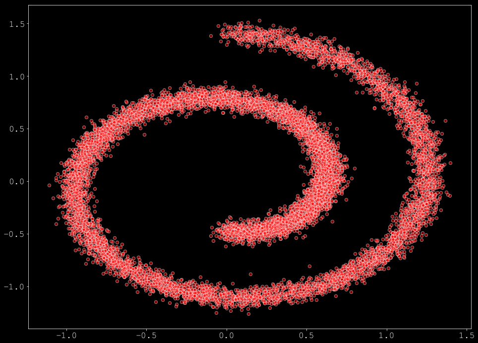
代码
文本
已隐藏单元格
代码
文本
[ ]
import torch
import torch.nn as nn
import torch.optim as optim
代码
文本
[1]
%matplotlib inline
import matplotlib.pyplot as plt
import numpy as np
from sklearn.datasets import make_swiss_roll

hdr_plot_style()
# Sample a batch from the swiss roll
def sample_batch(size, noise=0.5):
x, _= make_swiss_roll(size, noise=noise)
return x[:, [0, 2]] / 10.0
# Plot it
data = sample_batch(10**4).T
plt.figure(figsize=(16, 12))
plt.scatter(*data, alpha=0.5, color='red', edgecolor='white', s=40);
代码
文本

Score matching

Score matching aims to learn the gradients (termed score) of with respect to instead of directly . Therefore, we seek a model to approximate

We have seen that optimizing this model with an MSE objective was equivalent to optimizing

where denotes the Jacobian of with respect to . The problem with this formulation lies in the computation of this Jacobian, which does not scale well to high-dimensional data. This leads to a more efficient formulation of sliced score matching, which relies on random projections to approximate the computation of the Jacobian with

where are a set of Normal-distributed vectors. They show that this can be computed by using forward mode auto-differentiation, which is computationally efficient, as shown in the following implementation

代码
文本
[2]
import torch
import torch.nn as nn
import torch.optim as optim
def sliced_score_matching(model, samples):
samples.requires_grad_(True)
# Construct random vectors
vectors = torch.randn_like(samples)
vectors = vectors / torch.norm(vectors, dim=-1, keepdim=True)
# Compute the optimized vector-product jacobian
logp, jvp = autograd.functional.jvp(model, samples, vectors, create_graph=True)
# Compute the norm loss
norm_loss = (logp * vectors) ** 2 / 2.
# Compute the Jacobian loss
v_jvp = jvp * vectors
jacob_loss = v_jvp
loss = jacob_loss + norm_loss
return loss.mean(-1).mean(-1)
代码
文本

Denoising score matching

Originally, denoising score matching was discussed by Vincent [ 3 ] in the context of denoising auto-encoders. In our case, we can completely remove the use of in the computation of score matching, by corrupting the inputs through a distribution . It has been shown that the optimal network can be found by minimizing the following objective

An important remark is that is only true when the noise is small enough . As it has been shown in [ 3 ] , [ 8 ] , if we choose the noise distribution to be , then we have . Therefore, the denoising score matching loss simply becomes

We can implement the denoising score matching loss as follows

代码
文本
[3]
def denoising_score_matching(scorenet, samples, sigma=0.01):
perturbed_samples = samples + torch.randn_like(samples) * sigma
target = - 1 / (sigma ** 2) * (perturbed_samples - samples)
scores = scorenet(perturbed_samples)
target = target.view(target.shape[0], -1)
scores = scores.view(scores.shape[0], -1)
loss = 1 / 2. * ((scores - target) ** 2).sum(dim=-1).mean(dim=0)
return loss
代码
文本

Regarding optimization, we can perform a very simple implementation of this process, by define as being any type of neural network. We can perform the minimalistic implementation as follows

代码
文本
[4]
# Our approximation model
model = nn.Sequential(
nn.Linear(2, 128), nn.Softplus(),
nn.Linear(128, 128), nn.Softplus(),
nn.Linear(128, 2)
)
# Create ADAM optimizer over our model
optimizer = optim.Adam(model.parameters(), lr=1e-3)
dataset = torch.tensor(data.T).float()
for t in range(5000):
# Compute the loss.
loss = denoising_score_matching(model, dataset)
# Before the backward pass, zero all of the network gradients
optimizer.zero_grad()
# Backward pass: compute gradient of the loss with respect to parameters
loss.backward()
# Calling the step function to update the parameters
optimizer.step()
# Print loss
if ((t % 1000) == 0):
print(loss)
tensor(9996.8447, grad_fn=<MulBackward0>)
tensor(10036.8750, grad_fn=<MulBackward0>)
tensor(10104.2119, grad_fn=<MulBackward0>)
tensor(9976.1631, grad_fn=<MulBackward0>)
tensor(9974.6611, grad_fn=<MulBackward0>)
代码
文本

We can observe that our model has learned to represent by plotting the output value across the input space
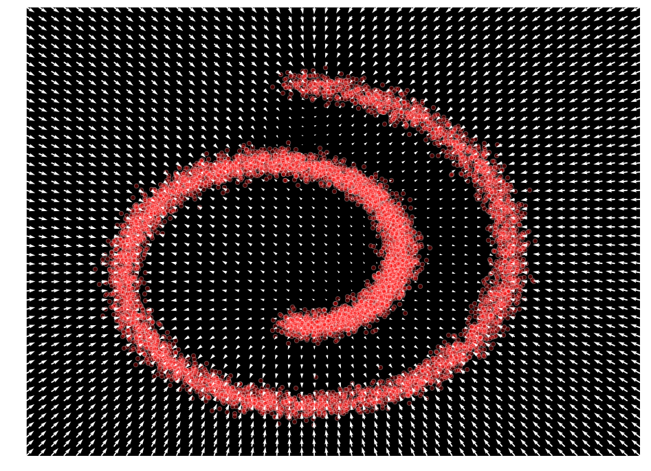
代码
文本
[5]
def plot_gradients(model, data, plot_scatter=True):
xx = np.stack(np.meshgrid(np.linspace(-1.5, 2.0, 50), np.linspace(-1.5, 2.0, 50)), axis=-1).reshape(-1, 2)
scores = model(torch.from_numpy(xx).float()).detach()
scores_norm = np.linalg.norm(scores, axis=-1, ord=2, keepdims=True)
scores_log1p = scores / (scores_norm + 1e-9) * np.log1p(scores_norm)
# Perform the plots
plt.figure(figsize=(16,12))
if (plot_scatter):
plt.scatter(*data, alpha=0.3, color='red', edgecolor='white', s=40)
plt.quiver(xx.T[0], xx.T[1], scores_log1p[:,0], scores_log1p[:,1], width=0.002, color='white')
plt.xlim(-1.5, 2.0)
plt.ylim(-1.5, 2.0)
plot_gradients(model, data)
代码
文本

Langevin sampling

We have also seen that Langevin dynamics is a process from thermodynamics that can produce true samples from a density , by relying only on

where and under : converges to an exact sample from . This is a key idea behind the score-based generative modeling approach.
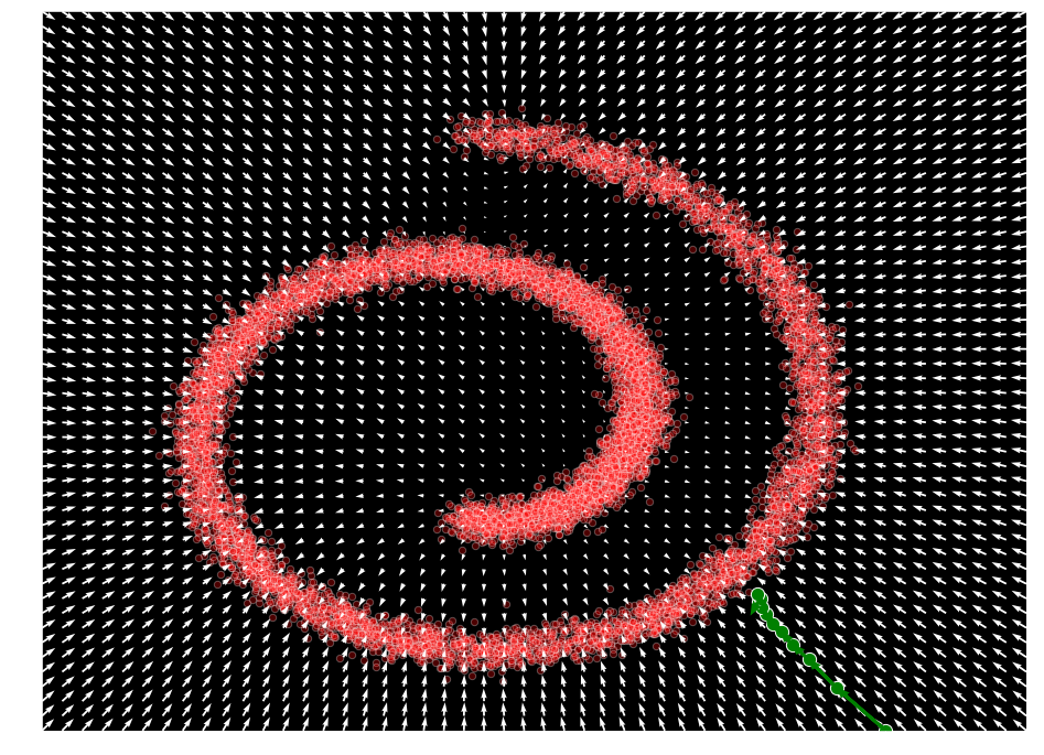
代码
文本
[6]
def sample_langevin(model, x, n_steps=10, eps=1e-3, decay=.9, temperature=1.0):
x_sequence = [x.unsqueeze(0)]
for s in range(n_steps):
z_t = torch.rand(x.size())
x = x + (eps / 2) * model(x) + (np.sqrt(eps) * temperature * z_t)
x_sequence.append(x.unsqueeze(0))
eps *= decay
return torch.cat(x_sequence)

x = torch.Tensor([1.5, -1.5])
samples = sample_langevin(model, x).detach()
plot_gradients(model, data)
plt.scatter(samples[:, 0], samples[:, 1], color='green', edgecolor='white', s=150)
# draw arrows for each mcmc step
deltas = (samples[1:] - samples[:-1])
deltas = deltas - deltas / torch.tensor(np.linalg.norm(deltas, keepdims=True, axis=-1)) * 0.04
for i, arrow in enumerate(deltas):
plt.arrow(samples[i,0], samples[i,1], arrow[0], arrow[1], width=1e-4, head_width=2e-2, color="green", linewidth=3)
代码
文本

Diffusion models

Diffusion probabilistic models were originally proposed by Sohl-Dickstein et al. [ 1 ] based on non-equilibrium thermodynamics. These models are based on two reciprocal processes that represent two Markov chains of random variables. One process that gradually adds noise to the input data (called the diffusion or forward process), destroying the signal up to full noise. In the opposite direction, the reverse process tries to learn how to invert this diffusion process (transform random noise into a high-quality waveform). This is examplified in the following figure, where we can see the whole model.

alt image.png

As we can see, the forward (and fixed) process gradually introduces noise at each step. Oppositely, the reverse (parametric) process must learn how to denoise local perturbations. Hence, learning involves estimating a large number of small perturbations, which is more tractable than trying to directly estimate the full distribution with a single potential function.

Both processes can be defined as parametrized Markov chains, but the diffusion process is usually simplified to inject pre-selected amounts of noise at each step. The reverse process is trained using variational inference, and can be modeled as conditional Gaussians, which allow for neural network parameterization and tractable estimation.

代码
文本

Formalization

Diffusion models are based on a series of latent variables that have the same dimensionality as a given input data, which is labeled as . Then, we need to define the behavior of two process

代码
文本

Forward process

In the forward process, the data distribution is gradually converted into an analytically tractable distribution , by repeated application of a Markov diffusion kernel , with a given diffusion rate .

This diffusion kernel can be set to gradually inject Gaussian noise, given a variance schedule such that

The complete distribution is called the diffusion process and is defined as

Here, we show how to perform a naive implementation of the simple forward diffusion process with a constant variance schedule

代码
文本
[7]
def forward_process(x_start, n_steps, noise=None):
""" Diffuse the data (t == 0 means diffused for 1 step) """
x_seq = [x_start]
for n in range(n_steps):
x_seq.append((torch.sqrt(1 - betas[n]) * x_seq[-1]) + (betas[n] * torch.rand_like(x_start)))
return x_seq
n_steps = 100
betas = torch.tensor([0.035] * n_steps)
dataset = torch.Tensor(data.T).float()
x_seq = forward_process(dataset, n_steps, betas)
fig, axs = plt.subplots(1, 10, figsize=(28, 3))
for i in range(10):
axs[i].scatter(x_seq[int((i / 10.0) * n_steps)][:, 0], x_seq[int((i / 10.0) * n_steps)][:, 1], s=10);
axs[i].set_axis_off(); axs[i].set_title('$q(\mathbf{x}_{'+str(int((i / 10.0) * n_steps))+'})$')
代码
文本

We can define any type of variance schedules for , as provided in the following function

代码
文本
[8]
def make_beta_schedule(schedule='linear', n_timesteps=1000, start=1e-5, end=1e-2):
if schedule == 'linear':
betas = torch.linspace(start, end, n_timesteps)
elif schedule == "quad":
betas = torch.linspace(start ** 0.5, end ** 0.5, n_timesteps) ** 2
elif schedule == "sigmoid":
betas = torch.linspace(-6, 6, n_timesteps)
betas = torch.sigmoid(betas) * (end - start) + start
return betas
代码
文本

Interestingly, the forward process admits sampling at an arbitrary timestep . Using notations and , we have

Therefore, we can update our diffusion sampling function to allow for this mecanism. Note that this depends on the given variance schedule of that we compute prior to the function.

代码
文本
[9]
betas = make_beta_schedule(schedule='sigmoid', n_timesteps=n_steps, start=1e-5, end=1e-2)
alphas = 1 - betas
alphas_prod = torch.cumprod(alphas, 0)
alphas_prod_p = torch.cat([torch.tensor([1]).float(), alphas_prod[:-1]], 0)
alphas_bar_sqrt = torch.sqrt(alphas_prod)
one_minus_alphas_bar_log = torch.log(1 - alphas_prod)
one_minus_alphas_bar_sqrt = torch.sqrt(1 - alphas_prod)
代码
文本

This allows to perform a very efficient implementation of the forward process, where we can directly sample at any given timesteps, as shown in the following code.

代码
文本
[10]
def extract(input, t, x):
shape = x.shape
out = torch.gather(input, 0, t.to(input.device))
reshape = [t.shape[0]] + [1] * (len(shape) - 1)
return out.reshape(*reshape)
def q_sample(x_0, t, noise=None):
if noise is None:
noise = torch.randn_like(x_0)
alphas_t = extract(alphas_bar_sqrt, t, x_0)
alphas_1_m_t = extract(one_minus_alphas_bar_sqrt, t, x_0)
return (alphas_t * x_0 + alphas_1_m_t * noise)
fig, axs = plt.subplots(1, 10, figsize=(28, 3))
for i in range(10):
q_i = q_sample(dataset, torch.tensor([i * 10]))
axs[i].scatter(q_i[:, 0], q_i[:, 1], s=10);
axs[i].set_axis_off(); axs[i].set_title('$q(\mathbf{x}_{'+str(i*10)+'})$')
代码
文本

Note that for training, we will also need to have access to the mean and variance of the posterior distribution of this process.

代码
文本
[11]
posterior_mean_coef_1 = (betas * torch.sqrt(alphas_prod_p) / (1 - alphas_prod))
posterior_mean_coef_2 = ((1 - alphas_prod_p) * torch.sqrt(alphas) / (1 - alphas_prod))
posterior_variance = betas * (1 - alphas_prod_p) / (1 - alphas_prod)
posterior_log_variance_clipped = torch.log(torch.cat((posterior_variance[1].view(1, 1), posterior_variance[1:].view(-1, 1)), 0)).view(-1)

def q_posterior_mean_variance(x_0, x_t, t):
coef_1 = extract(posterior_mean_coef_1, t, x_0)
coef_2 = extract(posterior_mean_coef_2, t, x_0)
mean = coef_1 * x_0 + coef_2 * x_t
var = extract(posterior_log_variance_clipped, t, x_0)
return mean, var
代码
文本

Reverse process

The generative distribution that we aim to learn will be trained to perform the reverse trajectory, starting from Gaussian noise to gradually remove local perturbations. Therefore the reverse process starts with our given tractable distribution and is described as

Each of the transitions in this process can simply be defined as conditional Gaussians (note: which is reminiscent of the definition of VAEs). Therefore, during learning, only the mean and covariancce for a Gaussian diffusion kernel needs to be trained

The two functions defining the mean and covariance can be parametrized by deep neural networks. Note also that these functions are parametrized by , which means that a single model can be used for all time steps.

Here, we show a naive implementation of this process, where we have a given model to infer variance. Note that this model is shared across all time steps but conditionned on that said time step.

代码
文本
[12]
import torch.nn.functional as F
class ConditionalLinear(nn.Module):
def __init__(self, num_in, num_out, n_steps):
super(ConditionalLinear, self).__init__()
self.num_out = num_out
self.lin = nn.Linear(num_in, num_out)
self.embed = nn.Embedding(n_steps, num_out)
self.embed.weight.data.uniform_()

def forward(self, x, y):
out = self.lin(x)
gamma = self.embed(y)
out = gamma.view(-1, self.num_out) * out
return out
class ConditionalModel(nn.Module):
def __init__(self, n_steps):
super(ConditionalModel, self).__init__()
self.lin1 = ConditionalLinear(2, 128, n_steps)
self.lin2 = ConditionalLinear(128, 128, n_steps)
self.lin3 = nn.Linear(128, 4)
def forward(self, x, y):
x = F.softplus(self.lin1(x, y))
x = F.softplus(self.lin2(x, y))
return self.lin3(x)
model = ConditionalModel(n_steps)
def p_mean_variance(model, x, t):
# Go through model
out = model(x, t)
# Extract the mean and variance
mean, log_var = torch.split(out, 2, dim=-1)
var = torch.exp(log_var)
return mean, log_var
代码
文本

As we can see, the reverse process consists in inferring the values of the mean and log variance for a given timestep. Then, once we have learned the correponding model, we can perform the denoising of any given timestep, by providing both the sample at a given time step, and that time step that we can use to condition the models for and .

代码
文本
[13]
def p_sample(model, x, t):
mean, log_var = p_mean_variance(model, x, torch.tensor(t))
noise = torch.randn_like(x)
shape = [x.shape[0]] + [1] * (x.ndimension() - 1)
nonzero_mask = (1 - (t == 0))
sample = mean + torch.exp(0.5 * log_var) * noise
return (sample)
代码
文本

Finally, obtaining samples from the model is given by running through the whole Markov chain in reverse, starting from the normal distribution to obtain samples from the target distribution. Note that this process can be very slow if we have a large number of steps, as we need to wait for a given to infer the following

代码
文本
[14]
def p_sample_loop(model, shape):
cur_x = torch.randn(shape)
x_seq = [cur_x]
for i in reversed(range(n_steps)):
cur_x = p_sample(model, cur_x, i)
x_seq.append(cur_x)
return x_seq
代码
文本

Model probability

The complete probability of the generative model is defined as

At first sight, this integral appears intractable. However, using a similar approach than variational inference, this integral can be rewritten as

代码
文本

Training

By using Jensen's inequality on the previous expression, we can see that the training may be performed by optimizing the variational bound on negative log-likelihood

Therefore, efficient training is allowed by optimizing random terms of with gradient descent.

To optimize this loss, we will need several computational tools, notably the KL divergence between two gaussians, and the entropy of a Gaussian.

代码
文本
[15]
def normal_kl(mean1, logvar1, mean2, logvar2):
kl = 0.5 * (-1.0 + logvar2 - logvar1 + torch.exp(logvar1 - logvar2) + ((mean1 - mean2) ** 2) * torch.exp(-logvar2))
return kl

def entropy(val):
return (0.5 * (1 + np.log(2. * np.pi))) + 0.5 * np.log(val)
代码
文本

Training loss

In the original paper by Sohl-Dickstein et al. [ 1 ] , this loss is shown to be reducible to

Hence, all parts of this loss can be quite easily estimated, as we are dealing with Gaussian distributions in all cases

代码
文本
[16]
def compute_loss(true_mean, true_var, model_mean, model_var):
# the KL divergence between model transition and posterior from data
KL = normal_kl(true_mean, true_var, model_mean, model_var).float()
# conditional entropies H_q(x^T|x^0) and H_q(x^1|x^0)
H_start = entropy(betas[0].float()).float()
beta_full_trajectory = 1. - torch.exp(torch.sum(torch.log(alphas))).float()
H_end = entropy(beta_full_trajectory.float()).float()
H_prior = entropy(torch.tensor([1.])).float()
negL_bound = KL * n_steps + H_start - H_end + H_prior
# the negL_bound if this was an isotropic Gaussian model of the data
negL_gauss = entropy(torch.tensor([1.])).float()
negL_diff = negL_bound - negL_gauss
L_diff_bits = negL_diff / np.log(2.)
L_diff_bits_avg = L_diff_bits.mean()
return L_diff_bits_avg
代码
文本

Training random time steps

The way that the model is trained is slightly counterintuitive, since we select a timestep at random to train for each of the batch input. The implementation taken from the DDIM repo provides a form of antithetic sampling, which allows to ensure that symmetrical points in the different chains are trained jointly. Therefore, the final procedure consists in first run the forward process on each input at a given (random) time steps (performing diffusion). Then we run the reverse process on this sample, and compute the loss.

代码
文本
[17]
def loss_likelihood_bound(model, x_0):
batch_size = x_0.shape[0]
# Select a random step for each example
t = torch.randint(0, n_steps, size=(batch_size // 2 + 1,))
t = torch.cat([t, n_steps - t - 1], dim=0)[:batch_size].long()
# Perform diffusion for step t
x_t = q_sample(x_0, t)
# Compute the true mean and variance
true_mean, true_var = q_posterior_mean_variance(x_0, x_t, t)
# Infer the mean and variance with our model
model_mean, model_var = p_mean_variance(model, x_t, t)
# Compute the loss
return compute_loss(true_mean, true_var, model_mean, model_var)
代码
文本

We can very simply optimize this loss with the following training loop.

代码
文本
[18]
model = ConditionalModel(n_steps)
optimizer = optim.Adam(model.parameters(), lr=1e-3)
dataset = torch.tensor(data.T).float()
batch_size = 128
for t in range(5001):
# X is a torch Variable
permutation = torch.randperm(dataset.size()[0])
for i in range(0, dataset.size()[0], batch_size):
# Retrieve current batch
indices = permutation[i:i+batch_size]
batch_x = dataset[indices]
# Compute the loss.
loss = loss_likelihood_bound(model, batch_x)
# Before the backward pass, zero all of the network gradients
optimizer.zero_grad()
# Backward pass: compute gradient of the loss with respect to parameters
loss.backward()
# Perform gradient clipping
torch.nn.utils.clip_grad_norm_(model.parameters(), 1.)
# Calling the step function to update the parameters
optimizer.step()
# Print loss
if (t % 1000 == 0):
print(loss)
x_seq = p_sample_loop(model, dataset.shape)
fig, axs = plt.subplots(1, 10, figsize=(28, 3))
for i in range(1, 11):
cur_x = x_seq[i * 10].detach()
axs[i-1].scatter(cur_x[:, 0], cur_x[:, 1], s=10);
axs[i-1].set_axis_off(); axs[i-1].set_title('$q(\mathbf{x}_{'+str(i*100)+'})$')
代码
文本

Denoising diffusion probabilistic models (DDPM)

In a very recent article, Ho et al. [ 1 ]  constructed over the diffusion models idea, by proposing several enhancements allowing to enhance the quality of the results. First, they proposed to rely on the following parameterization for the mean function

Note that now, the model is trained at outputing directly a form of noise function, which is used in the sampling process. Furthermore, the authors suggest to rather use a fixed variance function

This leads to a new sampling procedure for the reverse process as follows (we also quickly redefine the model to output the correct dimensionality).

代码
文本
[19]
class ConditionalModel(nn.Module):
def __init__(self, n_steps):
super(ConditionalModel, self).__init__()
self.lin1 = ConditionalLinear(2, 128, n_steps)
self.lin2 = ConditionalLinear(128, 128, n_steps)
self.lin3 = ConditionalLinear(128, 128, n_steps)
self.lin4 = nn.Linear(128, 2)
def forward(self, x, y):
x = F.softplus(self.lin1(x, y))
x = F.softplus(self.lin2(x, y))
x = F.softplus(self.lin3(x, y))
return self.lin4(x)

def p_sample(model, x, t):
t = torch.tensor([t])
# Factor to the model output
eps_factor = ((1 - extract(alphas, t, x)) / extract(one_minus_alphas_bar_sqrt, t, x))
# Model output
eps_theta = model(x, t)
# Final values
mean = (1 / extract(alphas, t, x).sqrt()) * (x - (eps_factor * eps_theta))
# Generate z
z = torch.randn_like(x)
# Fixed sigma
sigma_t = extract(betas, t, x).sqrt()
sample = mean + sigma_t * z
return (sample)
代码
文本

Notably, the forward process posteriors are tractable when conditioned on

And we can obtain the corresponding mean and variance as

代码
文本

Training in DDPM

Further improvements come from variance reduction by rewriting as a sum of KL divergences

All the KL divergences defined in this equation compare Gaussians, which means that they have a closed-form solution.

代码
文本
[20]
def approx_standard_normal_cdf(x):
return 0.5 * (1.0 + torch.tanh(torch.tensor(np.sqrt(2.0 / np.pi)) * (x + 0.044715 * torch.pow(x, 3))))

def discretized_gaussian_log_likelihood(x, means, log_scales):
# Assumes data is integers [0, 255] rescaled to [-1, 1]
centered_x = x - means
inv_stdv = torch.exp(-log_scales)
plus_in = inv_stdv * (centered_x + 1. / 255.)
cdf_plus = approx_standard_normal_cdf(plus_in)
min_in = inv_stdv * (centered_x - 1. / 255.)
cdf_min = approx_standard_normal_cdf(min_in)
log_cdf_plus = torch.log(torch.clamp(cdf_plus, min=1e-12))
log_one_minus_cdf_min = torch.log(torch.clamp(1 - cdf_min, min=1e-12))
cdf_delta = cdf_plus - cdf_min
log_probs = torch.where(x < -0.999, log_cdf_plus, torch.where(x > 0.999, log_one_minus_cdf_min, torch.log(torch.clamp(cdf_delta, min=1e-12))))
return log_probs
代码
文本

This leads to a new loss function as implemented in the following (note that this objective does not provide large change to the optimization itself).

代码
文本
[21]
def loss_variational(model, x_0):
batch_size = x_0.shape[0]
# Select a random step for each example
t = torch.randint(0, n_steps, size=(batch_size // 2 + 1,))
t = torch.cat([t, n_steps - t - 1], dim=0)[:batch_size].long()
# Perform diffusion for step t
x_t = q_sample(x_0, t)
# Compute the true mean and variance
true_mean, true_var = q_posterior_mean_variance(x_0, x_t, t)
# Infer the mean and variance with our model
model_mean, model_var = p_mean_variance(model, x_t, t)
# Compute the KL loss
kl = normal_kl(true_mean, true_var, model_mean, model_var)
kl = torch.mean(kl.view(batch_size, -1), dim=1) / np.log(2.)
# NLL of the decoder
decoder_nll = -discretized_gaussian_log_likelihood(x_0, means=model_mean, log_scales=0.5 * model_var)
decoder_nll = torch.mean(decoder_nll.view(batch_size, -1), dim=1) / np.log(2.)
# At the first timestep return the decoder NLL, otherwise return KL(q(x_{t-1}|x_t,x_0) || p(x_{t-1}|x_t))
output = torch.where(t == 0, decoder_nll, kl)
return output.mean(-1)
代码
文本

Simplifying loss to denoising score matching

The paper by Ho et al. [ 1 ] proposes a new parameterization for the mean of the reverse process Based on this parametrization, they show that the training objective can simplify to which resembles denoising score matching over multiple noise scales indexed by .

代码
文本

Further simplified training objective

The authors discuss the fact that it is beneficial to the sample quality to completely remove the complicated factor at the beginning of the loss. This further simplifies the objective as We can see that this objective now very closely ressemble the denoising score matching formulation. Furthermore, it provides an extremely simple implementation.

代码
文本
[22]
def noise_estimation_loss(model, x_0):
batch_size = x_0.shape[0]
# Select a random step for each example
t = torch.randint(0, n_steps, size=(batch_size // 2 + 1,))
t = torch.cat([t, n_steps - t - 1], dim=0)[:batch_size].long()
# x0 multiplier
a = extract(alphas_bar_sqrt, t, x_0)
# eps multiplier
am1 = extract(one_minus_alphas_bar_sqrt, t, x_0)
e = torch.randn_like(x_0)
# model input
x = x_0 * a + e * am1
output = model(x, t)
return (e - output).square().mean()
代码
文本

Stabilizing training with Exponential Moving Average (EMA)

This idea is found in most of the implementations, which allows to implement a form of model momentum. Instead of directly updating the weights of the model, we keep a copy of the previous values of the weights, and then update a weighted mean between the previous and new version of the weights. Here, we reuse the implementation proposed in the DDIM repository.

代码
文本
[23]
class EMA(object):
def __init__(self, mu=0.999):
self.mu = mu
self.shadow = {}

def register(self, module):
for name, param in module.named_parameters():
if param.requires_grad:
self.shadow[name] = param.data.clone()

def update(self, module):
for name, param in module.named_parameters():
if param.requires_grad:
self.shadow[name].data = (1. - self.mu) * param.data + self.mu * self.shadow[name].data

def ema(self, module):
for name, param in module.named_parameters():
if param.requires_grad:
param.data.copy_(self.shadow[name].data)

def ema_copy(self, module):
module_copy = type(module)(module.config).to(module.config.device)
module_copy.load_state_dict(module.state_dict())
self.ema(module_copy)
return module_copy

def state_dict(self):
return self.shadow

def load_state_dict(self, state_dict):
self.shadow = state_dict
代码
文本

The training loop is finally obtained with the following code

代码
文本
[24]
model = ConditionalModel(n_steps)
optimizer = optim.Adam(model.parameters(), lr=1e-3)
dataset = torch.tensor(data.T).float()
# Create EMA model
ema = EMA(0.9)
ema.register(model)
# Batch size
batch_size = 128
for t in range(1000):
# X is a torch Variable
permutation = torch.randperm(dataset.size()[0])
for i in range(0, dataset.size()[0], batch_size):
# Retrieve current batch
indices = permutation[i:i+batch_size]
batch_x = dataset[indices]
# Compute the loss.
loss = noise_estimation_loss(model, batch_x)
# Before the backward pass, zero all of the network gradients
optimizer.zero_grad()
# Backward pass: compute gradient of the loss with respect to parameters
loss.backward()
# Perform gradient clipping
torch.nn.utils.clip_grad_norm_(model.parameters(), 1.)
# Calling the step function to update the parameters
optimizer.step()
# Update the exponential moving average
ema.update(model)
# Print loss
if (t % 100 == 0):
print(loss)
x_seq = p_sample_loop(model, dataset.shape)
fig, axs = plt.subplots(1, 10, figsize=(28, 3))
for i in range(1, 11):
cur_x = x_seq[i * 10].detach()
axs[i-1].scatter(cur_x[:, 0], cur_x[:, 1], s=10);
#axs[i-1].set_axis_off();
axs[i-1].set_title('$q(\mathbf{x}_{'+str(i*100)+'})$')
代码
文本

Bibliography

代码
文本
notebook
Tutorial
Diffusion Model
notebookTutorial Diffusion Model
已赞1
推荐阅读
公开
Diffusion probabilistic models -03- Applications to waveforms
notebookEnglish Diffusion Model
喇叭花
发布于 2023-08-25
公开
Denoising diffusion probabilistic models-01-Score matching
EnglishnotebookTutorial Diffusion Model
喇叭花
发布于 2023-08-25
1 赞1 转存文件