快速开始 seaborn｜入门 seaborn 数据可视化

🎯 本教程旨在快速掌握使用 Seaborn 进行数据可视化的范式周期。

• 一键运行，你可以快速在实践中检验你的想法。

• 丰富完善的注释，对于入门者友好。

在 Bohrium Notebook 界面，你可以点击界面上方蓝色按钮 开始连接，选择 bohrium-notebook 镜像及任何一款节点配置，稍等片刻即可运行。

目标

入门 seaborn 进行数据可视化。

在学习本教程后，你将能够：

• 绘制统计估计、分布表示、分类数据的图表
• 使用 seaborn 对复杂数据集进行多元视图绘制
• 使用 seaborn 默认的绘图主题以及自定义你的主题

阅读该教程【最多】约需 15 分钟，让我们开始吧！

目录

• 背景
• 实践
  • 1 认识 seaborn
    • 1.1 什么是 seaborn
    • 1.2 安装 seaborn【Bohrium 中可直接运行，无需安装】
    • 1.3 验证安装并查看 seaborn 版本
  • 2 seaborn 方法
    • 2.1 快速入门示例
    • 2.2 用于统计图像
      • 2.2.1 统计估计
      • 2.2.2 分布表示
      • 2.2.3 分类数据的图表
    • 2.3 复杂数据集的多元视图
    • 2.4 默认风格和灵活的定制
  • 3 与 matplotlib 的关系
• 总结
• 进一步阅读
• 参考资料

背景

这是对 seaborn 的简短介绍，主要面向新用户。seaborn 是一个用于在 Python 中制作统计图形的库。它建立在 matplotlib 之上，并与 Pandas数据结构紧密集成。

你需要提前掌握以下知识：

• 非常基本的 Python 知识

实践

1 认识 seaborn

在这一部分，你会了解什么是 seaborn，在 Bohrium 中使用 seaborn，验证安装并查看版本。

1.1 什么是 seaborn

seaborn 是基于 Python 且非常受欢迎的图形可视化库，在 Matplotlib 的基础上，进行了更高级的封装，使得作图更加方便快捷。即便是没有什么基础的人，也能通过极简的代码，做出具有分析价值而又十分美观的图形。

seaborn 可以实现 Python 环境下的绝大部分探索性分析的任务，图形化的表达帮助你对数据进行分析，而且对 Python 的其他库（比如 Numpy/Pandas/Scipy）有很好的支持。

seaborn 官方文档对其能够绘制的各类图像进行了展示。

1.2 安装 seaborn

本教程是一个 Bohrium Notebook。Python 程序可直接在浏览器中运行，Bohrium 已安装 seaborn。

要按照本教程进行操作，请点击本页顶部的按钮，在 Bohrium Notebook 中运行本笔记本。

1. 你可以点击界面上方蓝色按钮 开始连接，选择 bohrium-notebook 镜像及任何一款计算机型，稍等片刻即可运行。

2. 若要运行笔记本中的所有代码，请点击左上角“ 运行全部单元格 ”。若要一次运行一个代码单元，请选择需要运行的单元格，然后点击左上角 “运行选中的单元格” 图标。

如果你的 Bohrium 镜像尚未安装 seaborn， 最方便的方法是通过 pip 安装:

如果你需要使用更特定于你的平台或包管理器的安装方法，你可以在这里查看更完整的安装说明。

1.3 验证 seaborn 安装并查看版本

安装 seaborn 后，确认库已成功安装并且你可以开始使用它。

不要跳过此步骤。

如果 seaborn 未正确安装或在此步骤中引发错误，则将无法运行之后的示例。

2 seaborn 方法

在这一节中，你会了解到一些 seaborn 的基础方法，包括：

• 一个快速入门示例
• 统计数据可视化
• 复杂数据的多元视图
• 默认风格与风格切换

2.1 快速入门示例

seaborn 是我们在这个简单示例中唯一需要导入的库。为了方便使用，使用 sns 作为缩写。

在幕后，seaborn 使用 matplotlib 来绘制其情节。对于交互式工作，建议在 matplotlib 模式下使用 Jupyter/IPython 界面，否则当您想查看绘图时，您必须调用 matplotlib.pyplot.show()。

这一步 matplotlib rcParam 系统，并且会影响所有 matplotlib 绘图的外观，即使您不使用 seaborn 制作它们。除了默认主题之外，还有其他几个选项，您可以独立地控制图的样式和缩放，以便在演示文稿上下文中快速转换您的工作（例如，制作一个版本的图，当在演讲期间投影时，字体可读）。如果您喜欢 matplotlib 默认设置或喜欢其他主题，则可以跳过此步骤并仍然使用 seaborn 绘图函数。

大多数文档中的代码将使用load_dataset()函数快速访问示例数据集。这些数据集没有什么特别之处：它们只是pandas dataframe，我们可以使用pandas.read_csv()加载它们或手动构建它们。文档中的大多数示例将使用pandas dataframe指定数据，但是seaborn对其接受的数据结构非常灵活。

这个图显示了使用单个调用seaborn函数relplot()在”tips“数据集中的五个变量之间的关系。请注意，我们仅提供了变量的名称和它们在图中的作用。与直接使用matplotlib时不同，不需要使用颜色值或标记代码来指定图形元素的属性。在幕后，seaborn处理了从数据框中的值到matplotlib理解的参数的转换。这种声明性方法使您可以专注于要回答的问题，而不是控制matplotlib的细节。

2.2 用于统计图像

没有普遍最佳的数据可视化方式。不同的问题最好由不同的图表来回答。seaborn通过使用一致的面向数据集的API轻松切换不同的可视化表示方式。

函数relplot()的名称是这样命名的，因为它旨在可视化许多不同的统计关系。虽然散点图通常很有效，但其中一个变量表示时间度量的关系更适合用线表示。relplot()函数具有方便的kind参数，可让您轻松切换到此备用表示方式：

请注意，size和style参数在散点图和线图中都有使用，但它们会以不同的方式影响两个可视化效果：在散点图中更改标记区域和符号，而在线图中更改线宽和虚线。我们不需要记住这些细节，让我们专注于图的总体结构和我们想要传达的信息。

2.2.1 统计估计

通常，我们对其他变量的平均值感兴趣。许多seaborn函数将自动执行必要的统计估计，以回答这些问题：

当估计统计值时，seaborn将使用bootstrapping来计算置信区间，并绘制代表估计不确定性的误差线1。

seaborn中的统计估计超出了描述性统计。例如，可以通过使用lmplot()来包含线性回归模型（及其不确定性）来增强散点图1。

2.2.2 分布表示

统计分析需要了解数据集中变量的分布。seaborn函数displot()支持多种可视化分布的方法，包括传统的直方图和计算密集的核密度估计。

seaborn 还推广一些强大但不太普遍的技术，例如计算和绘制数据的经验累积分布函数

2.2.3 分类数据的图表

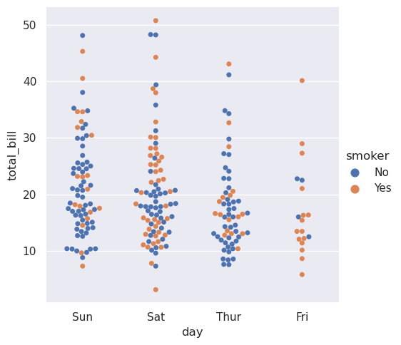
几种专门的seaborn绘图类型是面向可视化分类数据的。它们可以通过catplot()访问。这些图表提供不同级别的细化。在最细的级别上，您可能希望通过绘制“swarm”图来查看每个观察结果：这是一种散点图，它沿着分类轴调整点的位置，以便它们不重叠。”

或者，您可以使用核密度估计来表示从中抽样的点的基础分布

或者，您可以仅在每个嵌套类别中显示均值及其置信区间

2.3 复杂数据集的多元视图

一些 seaborn 函数结合多种绘图类型，以快速提供数据集的信息摘要。其中之一，jointplot()，专注于单个关系。它绘制两个变量之间的联合分布以及每个变量的边际分布:

另一个函数 pairplot() 则采用更广泛的视角：分别显示所有成对关系和每个变量的联合和边际分布:

2.3.1 用于构建图形的低级工具

这些工具通过将轴级绘图函数与管理图形布局的对象相结合，将数据集的结构链接到轴网格中。这两个元素都是公共API的一部分，您可以直接使用它们来创建只需几行代码即可创建复杂图形:

2.4 默认风格和灵活的定制

seaborn 是一个用于制作统计图形的库，它提供了一些默认的图形样式，但是也允许用户进行灵活的定制

seaborn通过单个函数调用创建完整的图形：在可能的情况下，其函数将自动添加信息轴标签和图例，以解释绘图中的语义映射。

在许多情况下，seaborn还将根据数据的特征选择其参数的默认值。例如，我们到目前为止看到的颜色映射使用不同的色调（蓝色，橙色，有时是绿色）来表示分配给色调的分类变量的不同级别。当映射数字变量时，某些函数将切换到连续梯度:

当你准备分享或发布你的作品时，你可能想要以比默认值更好的方式来打磨图形。seaborn 允许多个级别的自定义。它定义了多个内置主题，适用于所有图形，它的函数具有标准化的参数，可以修改每个绘图的语义映射，并且其他关键字参数传递到底层的 matplotlib 艺术家，允许更多的控制。一旦你创建了一个图，它的属性可以通过 seaborn API 和通过下降到 matplotlib 层进行精细调整来修改：

3 与 matplotlib 的关系

seaborn 与 matplotlib 的集成允许您在 matplotlib 支持的许多环境中使用它，包括笔记本中的探索性分析、GUI 应用程序中的实时交互以及多种栅格和矢量格式的归档输出。

虽然您可以仅使用 seaborn 函数来提高生产力，但完全定制您的图形需要一些 matplotlib 的概念和 API 知识。seaborn 新用户的学习曲线之一是知道何时下降到 matplotlib 层是必要的，以实现特定的自定义。另一方面，从 matplotlib 来的用户会发现他们的许多知识都可以转移。

Matplotlib 有一个全面而强大的 API；几乎可以更改图形的任何属性以满足您的喜好。seaborn 的高级接口和 matplotlib 的深度可定制性的组合将允许您快速探索数据，并创建可以定制为出版质量最终产品的图形。

Received message. seaborn 与 matplotlib 的集成允许您在 matplotlib 支持的许多环境中使用它，包括笔记本中的探索性分析、GUI 应用程序中的实时交互以及多种栅格和矢量格式的归档输出。 虽然您可以仅使用 seaborn 函数来提高生产力，但完全定制您的图形需要一些 matplotlib 的概念和 API 知识。seaborn 新用户的学习曲线之一是知道何时下降到 matplotlib 层是必要的，以实现特定的自定义。另一方面，从 matplotlib 来的用户会发现他们的许多知识都可以转移。 Matplotlib 有一个全面而强大的 API；几乎可以更改图形的任何属性以满足您的喜好。seaborn 的高级接口和 matplotlib 的深度可定制性的组合将允许您快速探索数据，并创建可以定制为出版质量最终产品的图形。

总结

在本教程中，您学习了在 seaborn 的一些基础方法。

具体而言，您了解到：

• 根据简单示例快速进行 seaborn 绘图
• 绘制统计估计、分布表示、分类数据的图表
• 使用 seaborn 对复杂数据集进行多元视图绘制
• 如何使用 seaborn 默认的绘图主题以及自定义你的主题

你有什么问题吗？ 欢迎与我们联系 bohrium@dp.tech 。

进一步阅读

如果您希望更深入学习 seaborn 及 Python 数据可视化，本节提供有关该主题的更多资源。

书籍

• Data Visualization in Python with Pandas and Matplotlib, 2021.

seaborn 项目

• seaborn Homepage.
• seaborn API Documentation
• seaborn, Wikipedia.
• seaborn on GitHub.

参考

1. https://seaborn.pydata.org/tutorial/introduction.html#lower-level-tools-for-building-figures
2. https://seaborn.pydata.org
3. https://github.com/seaborn/seaborn
4. https://zh.wikipedia.org/wiki/seaborn